Understanding Image Sharpness

– White Paper –

LumoLabs (fl)

Version:	Mar 13, 2012, v1.2
Status:	In progress
Print version:	www.falklumo.com/lumolabs/articles/sharpness/ImageSharpness.pdf
Publication URL:	www.falklumo.com/lumolabs/articles/sharpness/
Public comments:	blog.falklumo.com/2010/06/lumolabs-understanding-image-sharpness.html#comments

This White Paper is one in a series of articles discussing various aspects in obtaining sharp photographs such as obtaining sharp focus, avoiding shake and motion blur, possible lens resolution etc. This paper tries to provide a common basis for a quantitative discussion of these aspects.

1. Measures

Many authors use some form of test chart which contain high contrast lines with varying distance. Their distance is typically described as "lines per mm" where mm applies to the recording medium (sensor) rather than the test chart. In the digital age this head led to confusion because some people treated the background color as yet another line. In order to be precise, the test chart line density is now described by "line pairs per mm" or lp/mm or "cycles/mm" and means the same as lines per mm. The varying interpretation is now described by "line widths per mm" or LW/mm. 50 lp/mm and 100 LW/mm are the same.

In order to become independent on the size of the recording medium, all measures are often scaled to the image or picture height (PH). Esp. LW/PH is a popular unit and with a 35mm film or sensor, 100 LW/mm are 24 mm/PH ×100 LW/mm = 2400 LW/PH. LW/PH is often compared directly against the vertical pixel resolution of a sensor and many incorrectly believe that resolution measures cannot get larger than it. Another unit is "cycles/pixel" which is 0.5 when LW/PH equals the vertical number of pixels. This measure (0.5 cy/px) is sometimes called the Nyquist freqnency. Interestingly, the most naive measure (LW/px) is almost never seen in published material ;)

Below are a number of typical test charts which can be used for visual inspection of achievable resolution:

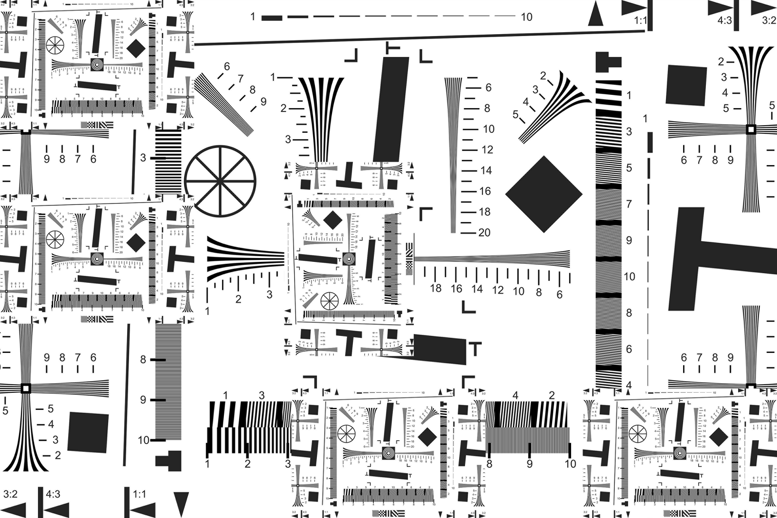
Fig. 1 ISO 12233 Test Chart as I use it. The inset parts are at 1/4x size. The numbers mean x100 LW/PH for the large part and x400 LX/PH for the small parts, both applicable if the chart spans the entire picture height. Some labs use a variant of the original chart with scales going to 40 rather than 20. But this is not sufficient for current high end cameras. A current high end Epson A2 inkjet printer can print the above chart to resolve to about the "60" mark ("15" in my inset parts).

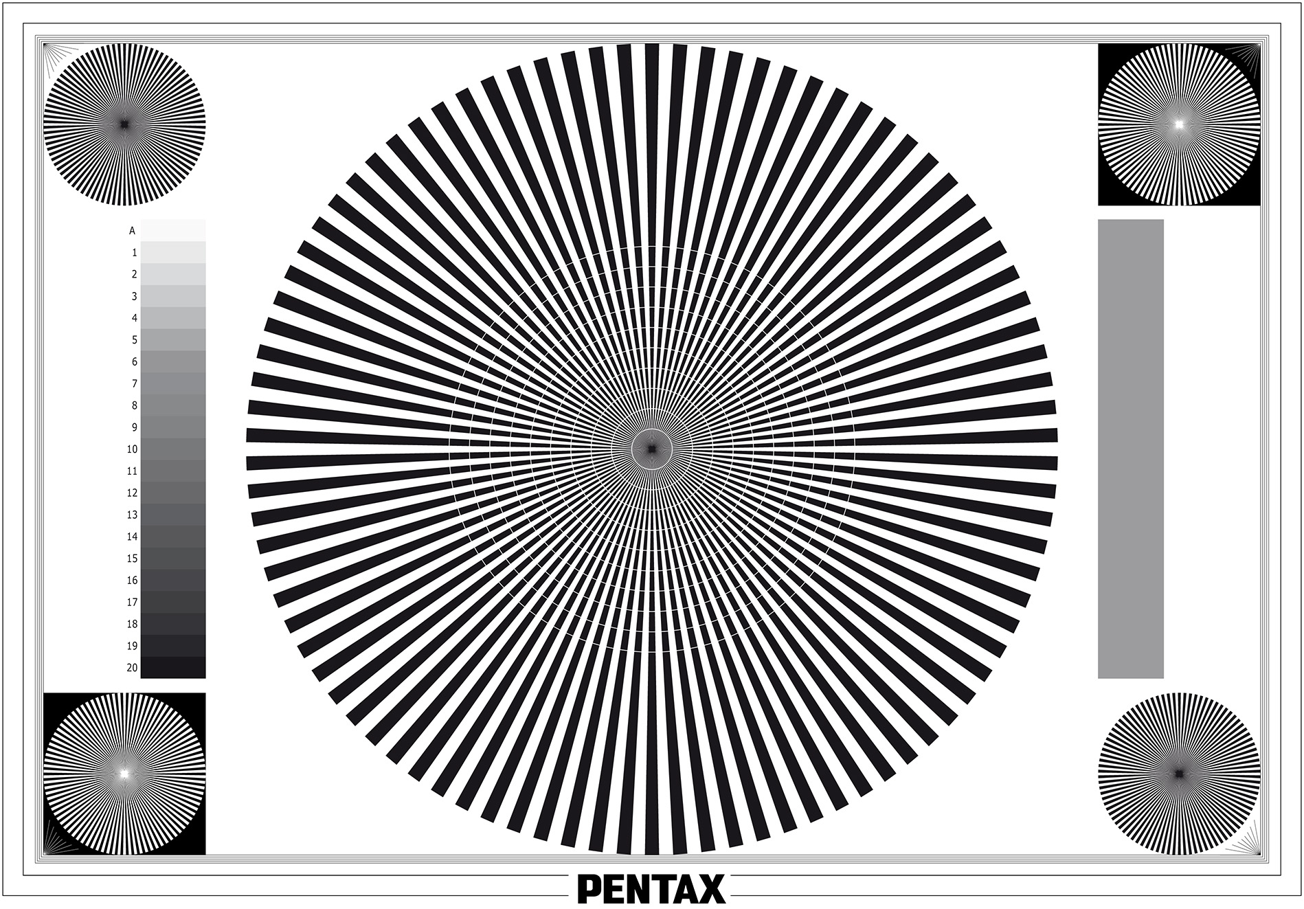
Fig. 2 Siemens star char. At least this is how this kind of test chart is called in Germany ;)

The artefacts in the middle of the chart are Moiré artifacts caused by resizing the original chart. Any photograph of the chart would contain much stronger artifacts.

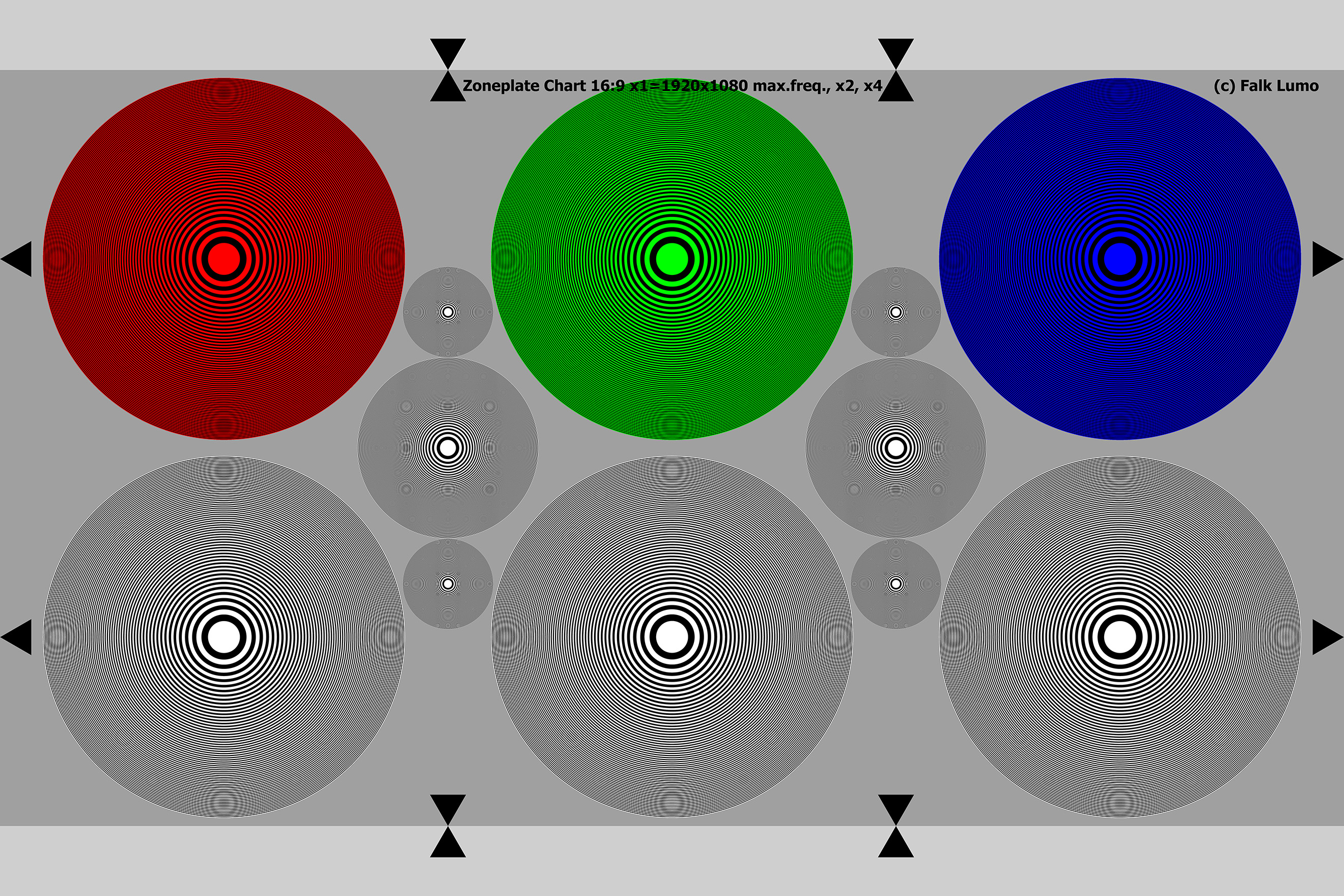
Fig. 3 Zone plate chart. Created to suit my needs. The 6 large zone plates have, at their outer border, a thin line distance corresponding exactly to 1080 LW/PH (when using the entire chart in a 3:2 frame or the marks within a 16:9 frame). The smaller plates correspond to up to 2160 LW/PH and 4320 LW/PH respectively. Unlike the Siemens star chart, the zone plate chart magnifies rather than minimizes the area of vanishing resolution.

A good recording system will just smear out detail when it cannot resolve it anymore. However, all digital recording systems I am aware of go beyond the edge of their capability and try to record in the lost signal domain. The purpose of the so-called anti-alias (AA) filter is to avoid this. This leads to clearly visible pseudo centers off the center of each zone plate and their exact location tells a lot about the recording process. Esp. The strength of an AA filter.

Esp. with subsampling video dSLRs, the above chart reveals the exact amout of line skipping in either direction. Esp. with Bayer filters, the Moiré areas have extreme or very dirty looking colors.

As nice as an evaluation of sharpness with test chart may appear, they can only provide subjective measures. E.g., look at the following crop from my 4x ISO 12233 inset:

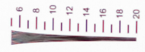
One may roughly estimate the resolution to be "6" (2400 LW/PH). Others may say "5.5" or "6.5" or even "7". And in a less obvious case one may be trapped by pseudo detail and say "10" while it really only is a Moiré artifact.

Therefore, a more quantitatively exact measure of sharpness was created a hundred years ago (or so).

1.1. Modular Transfer Function

The Modular Transfer Function (MTF) yields a number for any line pattern with given lp/mm. The black part and the white part of an extremely wide pattern (like upper half of the image being black, lower half being white) define the maximum possible difference of luminosities in any recording of the pattern. This difference is called 100% contrast, or 1. The distance between lines as given by the lp/mm figure is called the spatial frequency (or just frequency f) of the pattern. The contrast between black and white parts of the line pattern will decrease as the lines begin to smear out, the MTF number generally decreases as the frequency increases. A small detail: the mathematically correct line pattern will not be black and white but with sinusoidal gray levels in between, i.e., only the exact middle of a line is perfectly foreground and the exact middle between lines perfectly background. This MTF(f) function then is the accepted standard to measure sharpness or resolution.

Probably the best article about MTF is written by Hubert Nasse, Senior Scientist at Carl Zeiss AG. "Measuring lenses objectively - Why do we need MTF curves?" It is available online here: http://www.zeiss.com/C12567A8003B8B6F/EmbedTitelIntern/CLN_30_MTF_en/$File/CLN_MTF_Kurven_EN.pdf and http://www.zeiss.com/C12567A8003B8B6F/EmbedTitelIntern/CLN_31_MTF_en/$File/CLN_MTF_Kurven_2_en.pdf . Therefore, I confine myself within the scope of this article to what matters in our discussion.

So, first we observe that a single number cannot define sharpness. In almost all online discussions one treats resolution as a single number property but it isn't. Lens manufacturers typically provide MTF(f) across the image area (as it depends on the distance and orientation from the optical axis), giving it for selected discrete values for f, like 5/10/20/40 lp/mm (Leica) or 10/30 lp/mm (Sigma). The coarse-grain contrast (5 lp/mm) is generally associated to image contrast while the fine-grain contrast (40 lp/mm) is generally associated to image sharpness. Contrary to common belief, contrast and sharpness aren't the same.

When forced to single out a "resolution"-figure, we will often see a single frequency f where MTF(f) equals a given value, like 50%, 30% or 5%. These frequencies are often called f₅₀, f₃₀ or f₅, or MTF50, MTF30, or MTF5, respectively. For digital cameras, MTF50 is the most typically used value and often given in LW/PH. E.g., photozone.de uses this convention when giving lens resolution figures. In the film era, MTF30 was more normal and I would say that analog MTF30 and digital MTF50 figures should be compared directly as the former applies sharpening (cf. below) and the latter doesn't. Finally, MTF5 is an important figure too when it comes to the limiting resolving power of a lens, e.g., for information extraction. E.g., Zeiss quotes an MTF5 figure of about 300 lp/mm center resolution for their 35mm SLR prime mount lenses.

Why is all of this important? Because we need it when studying the cummulative effect of various sources of "blur". We need to understand how to define "blur" and how it "adds" from various sources.

1.2. Blur

In its most simple form, we can consider blur to be the inverse of resolution. E.g., if some MTF50 figure reads 50 lp/mm (100 LW/mm) then we could say the blur is 1/100 mm or 10 µm (or 2 pixels with 5 µm pixels).

However, we can define all this in a much more precise way. As it turns out, the MTF(f) function is the Fourier transform of the Line Spread Function (LSF) which in turn is the first derivate of the Edge Spread Function (ESF). The properties of the LSF can be derived from the Point Spread Function (PSF). The PSF is nothing but the image of a point like source like a star at a starry night. Astro photographers often define sharpness as the amount of light energy falling onto the Airy disc (compared to a diffraction-limited optics) and call it Strehl ratio. An "80% Strehl" is considered good. ;)

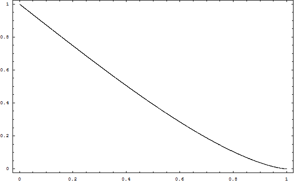
The LSF is the image of a single line. Below is a graph of such a line image:

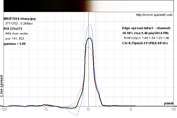As you can see, the line isn't exactly recorded by a stair case function. There is a certain amount of smearing. An ideal LSF (of a 1 pixel wide line) would be 100% between -0.5 and +0.5 pixels and 0% elsewhere. A pixelating sensor cannot record lines finer than 1 pixel width with full contrast.

As it turns out, the surface under the LSF and the MTF50 value are related in a simple way. Not mathematically exactly, but for most practical purposes. In order to explain, we study several cases, from most simple to real cases.

1.2.1. The hard pixel

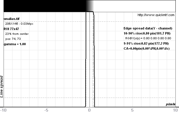
This is the hard pixel's stair case LSF as discussed above. Note however that this kind of pixel needs to an ugly aliasing "stair case" effect along edges in the image as shown above. Before we discuss the consequence of eliminating this effect, let's first understand the properties of an image made of "hard" pixels. So, we now show both the corresponding ESF and MTF.

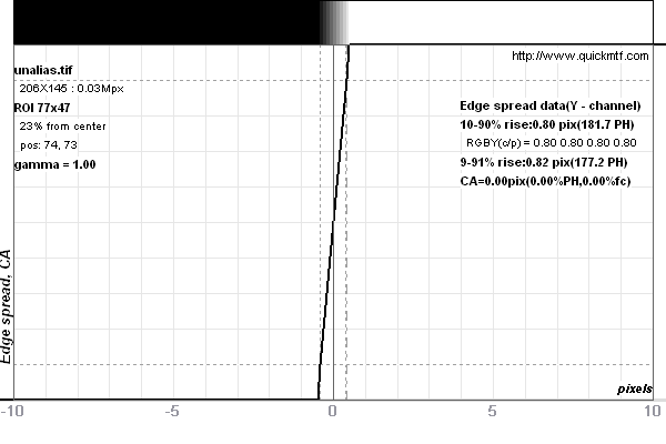
Despite the hard pixel, the edge isn't infinitely steep. It's slope must be a finite 1/pixel because the LSF is its derivate.

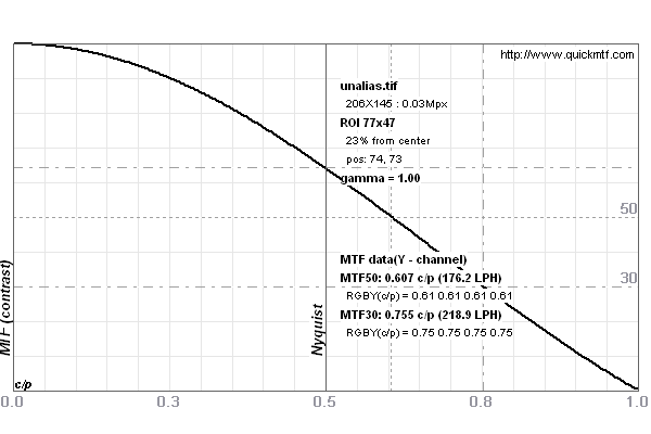
It is common practice to characterize an edge by the distance between 10% and 90% luminosities, the so-called "10-90% edge blur width". For the hard pixel, we can easily compute it exactly: 0.80 pixels (0.90-0.10). It is however, a bit harder to compute the hard pixel's MTF50 value. Above is the MTF(f) curve where f is given in cy/px. We already discussed this unit and 0.5 cy/px corresponds to 1 LW/px and is the Nyquist limit. MTF(f) is the Fourier transform of the LSF and can be solved in closed form (for f given in cy/px):

MTF(f) = sinc(π f) where sinc(x) := sin(x)/x is the sinus cardinalis

therefore MTF(0.5 cy/px) = 2/π or ≈0.6366 and MTF50=0.6033545644... This means that the MTF50 value corresponds to the numeric edge blur for a 82.87% rise (0.5/MTF50) or an edge rise from 8.565% to 91.435%, the "9-91% edge blur width".

In practice, it turns out that this equivalence relation between the 9-91% edge blur width and the MTF50 frequency is quite generic. Many authors use both measurements in an interchangeable way and most replace the 9-91% edge blur width by the 10-90% edge blur width in doing so. The advantage of the 10-90% edge blur widthis that it is easily visualized and understood: It means how thin an edge appears on screen. MTF50 is a frequency (like cy/px) and its inverse is a length (like px/cy). Half this length (half cycle) is the blur width b ≈0.5/MTF50.

Another advantage is that it is easily measured by the 5° slanted edge method. Affordable software exists to do the numeric evaluation, e.g., QuickMTF from Kiev (http://www.quickmtf.com). Below is the corresponding test chart:

Fig. 4 Slanted edge test chart. It is best to print an unslanted version (as shown above) and mount/photograph at a 5° angle. There are alignment bars in the chart above to facilitate the alignment. Because a few hundred pixels suffice to measure an edge with better than 0.1px subpixel accuracy, there is no need to print the above chart big. Just print on A4 sheet and photograph from a distant wall.

A zone plate chart allows for more accurate manual focussing in live view mode. So, a combination of both may provide best results.

1.2.2. The perfect pixel

As mentioned above, the hard pixel isn't perfect as it renders staircase edges. We define the perfect pixel to be one which collects exactly as much light as the bright part of the pattern covers. This is what downsizing with bilinear resampling would provide when starting with an extremely high resolution image made of hard pixels.

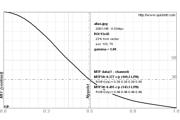
This makes the stair case effect invisible but as you can see, at the expense of measured sharpness. MTF50 is now 0.377 cy/px and 10-90% edge blur width is 1.26 px. Again, the 9-91% rise provides the same resolution figure as MTF50 does.

Note: Whenever you see an edge blur width of less than 1.26 pixels or an MTF50 resolution of more than 75.4% of vertical pixels (2340 LW/PH in the case of 3104 vertical pixel resolution like a Pentax K-7) then this beats the perfect pixel perfomance, i.e., a theoretically perfect camera system. This applies to system performance. Single lens performance can be better when measured on an optical bench. If you look at photozone.de then you see that e.g., the Pentax FA31 Ltd. lens at f/4 renders 2345 LW/PH. And this with a sensor which has a perfect pixel limit of 1954 LW/PH... To understand this phenomen, we have to proceed.

A good (albeit not exact) approximation of the MTF(f) function for the perfect pixel is the square (or cube) of the MTF(f) function for the hard pixel. All we need to remember for the time being is the S-shaped form of the MTF(f) function. With

MTF(f) = sinc^p(πf)

we obtain MTF50 = 0.443(0.366) cy/px or a blur width of 1.13(1.37) px for p=2(3).

1.2.3. The real pixel, sharp and soft

The real pixel as we find it in our actual photographs when pixel peeping is only approximately like the perfect pixel.

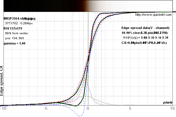
This is an example of a real edge captured with a Bayer Sensor (Pentax K-7 with DA*60-250/4 at 250mm f/5.6 1/180s out of Lightroom). There is a bit color aberration which is why the edge doesn't look perfectly gray. The 10-90% edge blur width is 1.36 px (the steeper curve in the left plot above) and MTF50 is 0.35 cy/px (the upper curve in the right plot above). Both is very close to the perfect pixel indeed. Again, 9-91% rise and MTF50 match. One may say that all pixels of the sensor are turned into information.

However, this result depends more on development parameters than on anything else. The development parameters are the following Lightroom (v2.5) settings: default parameters (Brightness: 50, Contrast: 25, Tone curve: Medium) plus sharpening (Amount: 100, Radius: 0.5, Detail: 25, Masking: 0). I will refer to the above parameters as the "Sharp setting".

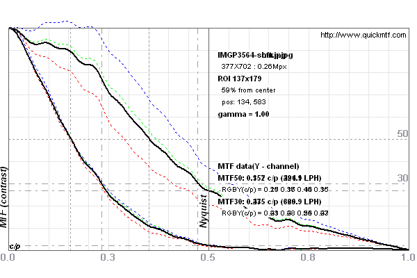
When parameters are changed to linear setting (as they really come out of the sensor): (Brightness: 0, Contrast: 0, Tone curve: Linear) without sharpening (Amount: 0) then the other two curves are obtained in the two plots above. I will refer to the linear parameters as the "Soft setting".

The numeric values are 3.37 px 10-90% edge blur width and MTF50 is 0.16 cy/px. This is only half the resolution – for the exact same image! BTW, the MTF50 value now relates to the 11-89% rise and simplifying the rule of thumb to 10-90% is ok if soft images are considered too.

Note: MTF measurements as published on the web are more than everything else, measurements of the applied sharpening settings. As there is no standard for these settings, MTF50 values from different sources cannot be compared. The difference of edge blur widths may still be significant though as we will discuss in a second. Also, measurements of lens MTFs obtained on an optical bench are comparable as all luminosities are to be recorded linearly and without applying a spatial filter then.

Now, we easily understand how MTF50 figures beating the perfect pixel can exist: It simply is a result of oversharpening. Even our Sharp setting is rather moderate as it uses a small Radius of 0.5 px only. Sharpening can be done much more aggressively and many testers seem to do so.

All we need to remember for the time being is that the Sharp setting yields an S-shaped MTF(f) function too. The Soft setting does not.

1.3. More realistic resolution measures

I am not satisfied that resolution measurements are sharpening measures. Quoting MTF50 was ok when it was a direct analog measures of optical performance. Not anymore. So, we at Lumolabs are researching alternative measures. One is the blur momentum (ZBM and FBM):

where m=0 for the zeroth blur moment ZBM and p=1 for the first blur moment FBM. The following holds true for the hard pixel: mth BM(hard)=1/2 for all m. The delta_lum integrand means the (minimal) deviation of edge luminosity from an ideal edge step function {0, 1} and px the distance from the edge position measured in pixels.

Let's look at images of the respective image qualities (to the right). This shows a hard, perfect and sharpened edge, from left to right, respectively. The corresponding 10-90% rise widths are 0.80 px, 1.24 px and 0.81 px resp. We rather would prefer a measure which ranks the (over)sharpened edge last. The hard pixel will always win whatever be its measure. But for the other two, we get: ZBM(perfect/sharpened)=0.79/0.74 px and FBM(perfect/sharpened)=1.43/2.11 px². The following chart shows the ZBM integral over px and how both end up to be about the same (6% difference).

For pragmatic reasons, we currently propose to additionally measure and quote ZBM and to avoid full white or full black in test charts. However, more research is required and several sample images with different levels of sharpening applied should be studied.

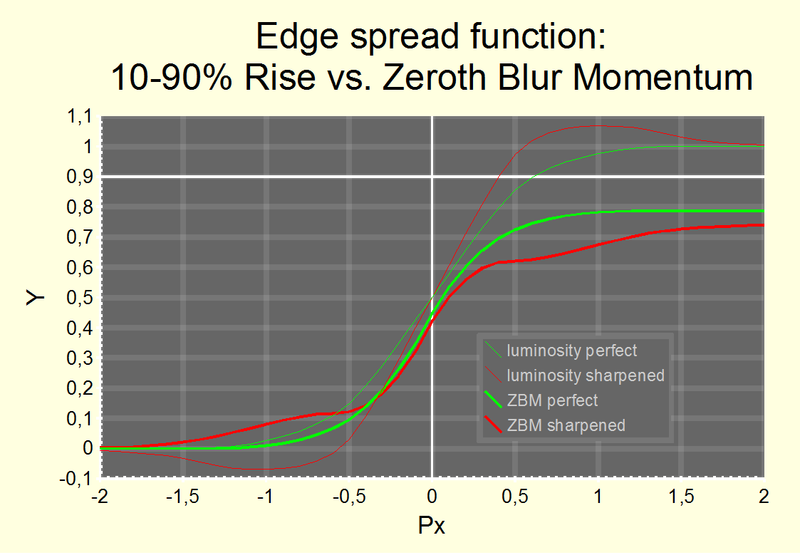
Fig. 5 Comparison of Zeroth Blur Momentum ZBM for a perfect edge and a perfect edge further sharpened with USM radius 0.5 px.

The sharpening does almost not affect the ZBM measure which in both cases is about the same ratio compared to the hard pixel as for the 10-90% perfect pixel rise width. So, 1.6 x ZBM can directly replace the 10-90% rise width.

1.4. Combining blur

At the heart of this paper is the question how blur from different sources (or causes) combines. This is a question not typically addressed. We need to overcome this if we really want to understand image sharpness.

The first time a ran across this question was by somebody citing the "Kodak formula":

1/r = 1/r_film + 1/r_lens

where r was the resolution and in the context of this paper, should be read to mean MTF30. Unfortunately, no argument was provided for this formula. Our equivalence of 10-90% edge blur width b and MTF50 can be used to rewrite the Kodak formula like this:

b^p = b^p_film + b^p_lens

where p=1 is the exponent in a generalized Kodak formula. While I've seen the Kodak formula cited with p=2, I must say that the reality is a bit more complex than this.

First of all, let's accept that there is no a-priori reason why blur parameters should be combinable in any easy way. An optical system with a series of processing steps (lens, AA filter, color filter, sensor, time integration, digital postprocessing) is mathematically described as a series of convolutions of the input signal with the PSF or LSF of the respective step. Convolution is a well known mathematical operation and its inverse is called Deconvolution. Just think of a convolution as of a Photoshop filter operation, like the application of the "Gaussian blur" filter.

As mentioned, the nice thing about the MTF is that it is the Fourier transform of the LSF. So, rather than convolving all those LSFs, we can simply multiply all MTFs together.

The problem is that in general, if we multiply two functions MTF(f) which are parametrized by two parameters, then MTF₁(f)×MTF₂(f) is not a function described by the same parameter, i.e., the MTF50 value of the product isn't easily computed from the respective MTF50 values of the factors.

There is one class of functions which are an exception, exponential functions:

exp(-c f^p × 1/r₁^p) × exp(-c f^p × 1/r₂^p) = exp (-c f^p × (1/r₁^p + 1/r₂^p))

which is the Kodak formula for arbitrary p. So, the Kodak formula for exponent p is applicable if MTF(f) for 0<f<f₅₀ for both factors roughly looks like exp(-f^p). Now, the curve with p=1 looks like the radioactive decay curve (no S shape) and the curve with p=2 looks like one half of the Gaussian normal distribution curve (yes S shape). We simplify this into the following rule:

b = b₁ + b₂ if MTF₁ and MTF₂ are both mainly concave up to the larger f₅₀ values.
b² = b₁² + b₂² if MTF₁ and MTF₂ are both mainly S-shaped.
This is an RMS (root mean square) treatment for blur terms.

The following chart compares a number of parameterized functions to model MTF(f):

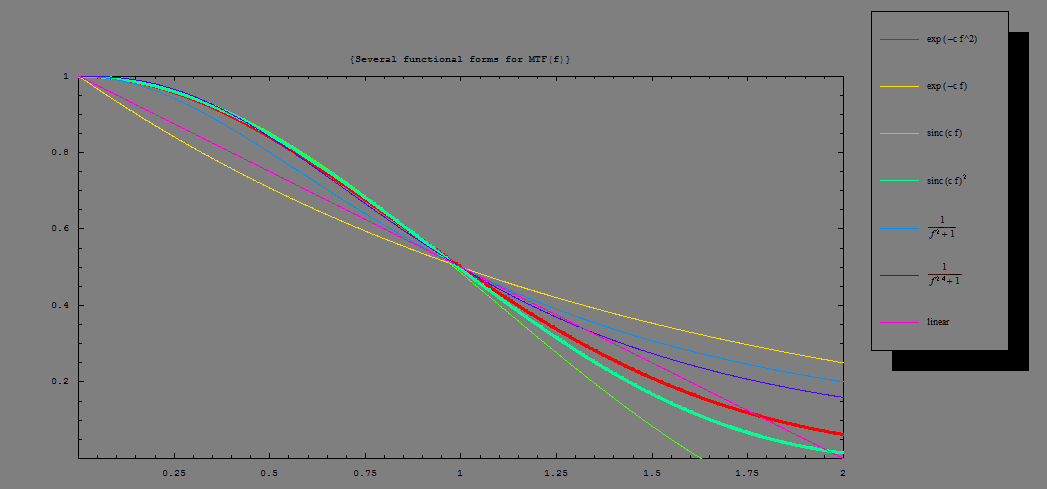
Fig. 6Comparison if various MTF(f) functions with equal MTF50 (f₅₀) value. The first (thick red) curve corresponds the Gaussian curve (where p=2applies) and the fourth (thick green) curve corresponds the squared sinus cardinalis roughly describing the perfect pixel. Both match well up to f₅₀, as does the sinus cardinalis (third line, green) describing the hard pixel and 1/(1+f^2.4)(sixth line, dark blue).

Note that a popular form 1/(1+f²) (fifth line, bright blue) doesn't fit an easy treatment, as does a linear form as is sometimes assumed (e.g., in the paper by H. Nasse). Such cases as well as the MTF we saw for the "Soft setting" is better fitted by a simple exponential (second curve, yellow) and should be treated with p=1, i.e., by the original Kodak formula. If only one curve is S-shaped, we recommend to rather use the original Kodak formula p=1.

In the following, we will combine blur widths by sometimes adding them linearly, sometimes by their square. You just saw the reasoning behind it.

Of course, this calculus is most useful to single out individual component performance figures, like lens performance before blur due to sensor pixellation and diffraction. Just keep in mind that the calculus is approximative only.

2. Sources of blur

In this chapter, we discuss and compare various sources of blur in an image.

Here, we will express lengths in µm (rather than dimensionless px) and frequencies in cy/µm rather than cy/px.

px→ length / ρ

f_old → f ρ

where ρ is the pixel pitch.

2.1. Bayer matrix, anti aliasing and sharpening

The anti alias filter in front of the sensor (to avoid Moiré patterns) and the Bayer color filter with demosaicing algorithm to interpolate local RGB values from the local and neighboring color channel values creates a loss of sharpness. The AA filter shouldn't be considered to be independent from the Bayer filter too. As Moiré artifacts with a Bayer filter have extreme false color w/o an AA filter which remain visible from a distance even if the Moiré pattern does not.

The reason is that a sensor with Bayer color filter has a lower spatial resolution in the color channels than it has in the luminosity channel. Therefore, in order to make each color sensor receive sufficient color information, each ray is split into 2x2 rays which are (for a full or so-called "strong" AA filter) separated by the pixel distance. This is typically done with a pair of lithium niobate crystals turned 90° against each other. Note that the lithium niobate beam splitter is no anti alias or low pass filter! The common talk to name this device a "camera's AA filter" is technically not correct. The pixel structure itself including the microlens array serves as a low pass filter where a pixel with 100% fill factor (i.e. which is light sensitive across its entire surface due to its micro lens) does an anti-alias integration over its surface.

We'll call the additional beam splitter the Bayer-AA filter or just the "BAA filter".

The MTF for such integration over a pixel was already given above, in section 1.2.1 on page 6:

MTF (f) = sinc (πf ρ)

The beam-splitter causes integration over twice the pixel pitch:

MTF_AA(f) = sinc (2 πf ρ) = cos (πf ρ) sinc (πf ρ)

MTF_BAA(f) = MTF_AA (f) / MTF (f) ) = cos (πf ρ)

MTF_BAA describes the additional effect of the Bayer-AA filter. It is 0 at f = 1/(2 ρ) and b_BAA = 0.5/f₅₀ becomes exactly (for a "strong AA" filter):

b_BAA= 1½ ρ (for a strong BAA filter)

The extra blur caused by the micro-lenses' pixel integration alone (rendering a perfect pixel) was given in section 1.2.2 as the increase in blur width from 0.8 px to 1.26 px which is (using the Kodak formula with p=2):

b_AA = 1 ρ

The combined effect b_AA+BAA≈ 1.8 ρ and the resulting pixel blur of a Bayer pixel is ≈ 2.0 ρ.

Of course, this is difficult to measure if there aren't two versions of the camera available: the color one and a monochrome one w/o BAA filter. Sometimes, the choice exists as monochrome cameras w/o BAA filter are offered for astro photography. But not in general. Another nice test could be with a Foveon X3 sensor which has no Bayer-AA filter. More on this with some nice MTF tests is found here: http://www.foveon.com/files/ResolutionforColorPhotography.pdf .

The matter is complicated further by the fact that contrast (as long as it isn't zero or almost zero) can be recovered using sharpening techniques. Direct case to case comparisons lack to pay proper credit to this fact. In the discussion above, we have seen that many MTFs become (almost) zero at about twice the f₅₀ frequency. This isn't a universal fact but for many natural MTF functions (hard pixel, BAA filter, diffraction, defocus) this is a good rule of thumb.

This means that sharpening can almost half the blur widths in an image, say, reduce them by 1/3 in practice. As long as the image noise is small at the given spatial frequency (low ISO in current dSLRs do the trick) and the resulting blur width stays above ≈ 1.25 ρ, this is achievable without significant artefacts.

Therefore, sharpening an otherwise perfect image can cancel the effect of a Bayer-AA filter (reducing the blur from ≈ 2.0 ρ to ≈ 1.3 ρ which is a 1/3 reduction). Sometimes, this method is preferrable over post-processing the Moiré and false specular color artefacts created by a missing BAA filter.

The complication is that as a consequence, a camera with a Bayer sensor is almost always combined with sharpening. This makes the blur analysis a bit awkward.

I decided to evaluate the effect in a very pragmatic way. As has been seen, the "Sharp setting" of the Lightroom development process roughly compensates for the effect of the BAA. And the "Soft setting" is believed to better represent the raw data as recorded by a sensor. Therefore, the difference of resolution figures from the Soft and Sharp settings are believed to represent the amount of undone blur cancellation due to the BAA filter.

Maybe this is wrong. But let us study the difference anyway. If not the effect of BAA filtering it at least will showcase the effect of sharpening.

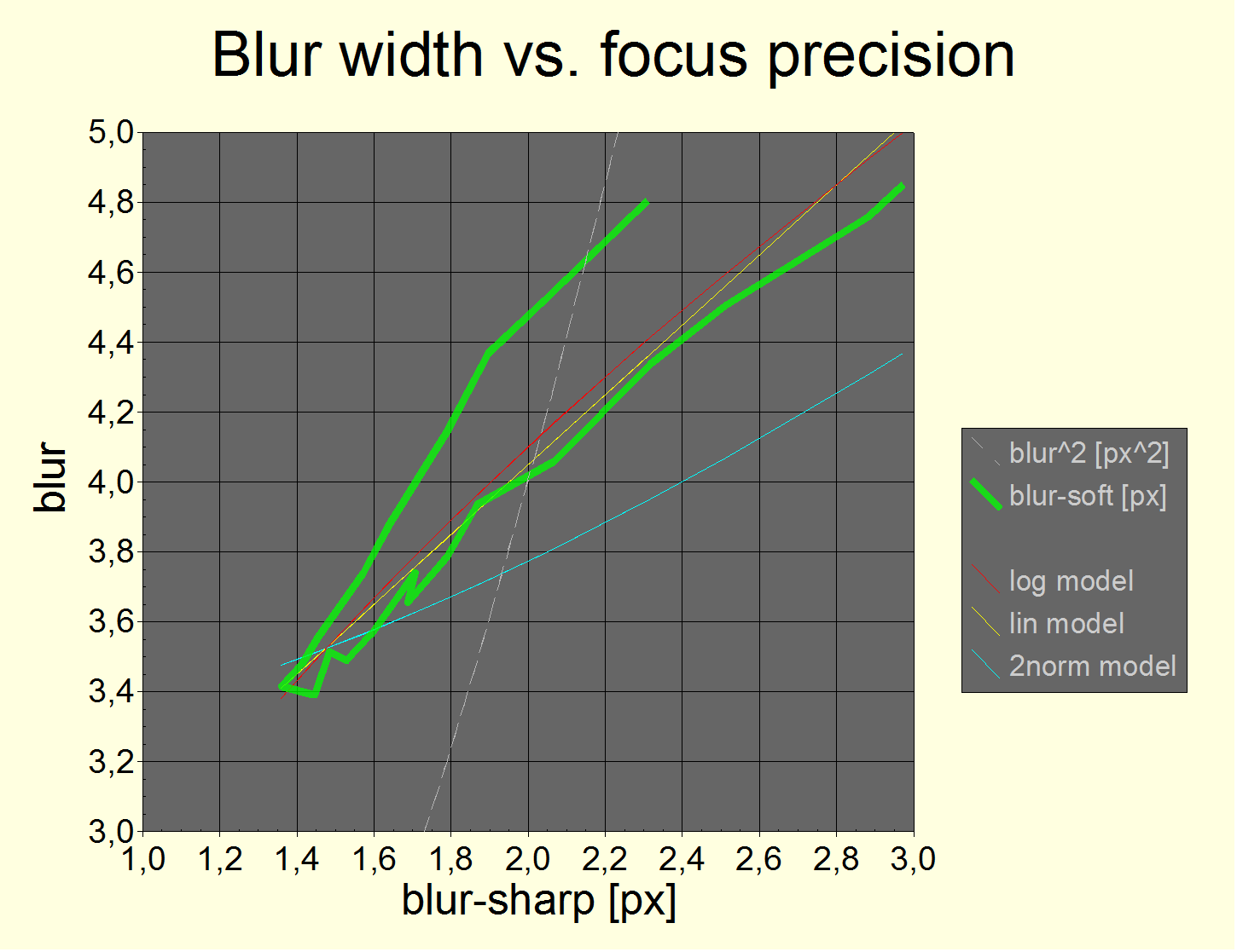
Fig. 7 Blur width of the "Soft setting" vs. blur width of the "Sharp setting" (fat green line). Note that only the Lightroom development settings are different! The accepted combination formula is the Kodak formula with p=1 (yellow line) while p=2 delivers a bad fit (blue line). As to be expected from the concave form of the MTF curve for the "Soft setting".

The red line represents a power law (with exponent ½) which delivers very similiar results.

The fat green line is a 2D curve because the blur was produced by travelling from backfocus to exact to frontfocus. As one can see, the same amount of blur for the sharp setting produces slightly different amounts of blur for the soft setting for front and backfocus, resp. Where backfocus has more soft blur than front focus. This is explained by a reversal of color aberrations when going from back to frontfocus and a nonlinear response curve for different colors and luminosities.

In this kind of sharp vs. soft blur plot, the point of exact focus is much more visible than in the blur vs. shift plot of fig. 14.

The effect of the Soft setting is best described by linearly adding a "non-sharpening" blur

b_soft= 2.05 ρ (add blur linearly as the last step)

to the blur values of the Sharp setting. At least with a Pentax K-7 camera. It slightly varies with different lenses and scenarios but not by much.

Needless to say that 2 px difference is huge ;) The sharpening seems to undo more than just the Bayer-AA filter blur which should only account for about half the effect (cf. above).

2.2. Diffraction

The quantum nature of photons implies that you can't simultaneously know their direction and position. This does not only severely limit the resolution of a light field camera such as the Lytro cameras. But any lens aperture provides an imprecise measure of a photon's position and this implies that their direction such as measured by their detection on a recording plane will smear. The better the measurement of position (i.e., the smaller the lens aperture) the larger the smear.

The smear (the diffraction PSF) looks like the image to the right. A central region with most of the luminosity (84%) is bound by a first ring with null intensity. The central region is called the "Airy disk". It has a radius (half diameter) of

r_Airy = 1.22 λ N

where λ is the wavelength of light (e.g., 0.55 µm for green light) and N is the aperture's f-stop number, the ratio of focal length / aperture diameter.

The Rayleigh criterion defines the limiting resolution by a line pattern where two line pairs are r_Airy apart. The true limit though is

f₀= 1 / (λN)

which is the frequency of zero MTF. The full MTF is:

MTF_diff (f) = 2 / π(arccos(k) - k √(1 – k²)) with k = f/f₀= f λN

Note that here we use an alternative way to specify spatial frequencies (in terms of dimensionless kor units of f₀) as we work independently from a pixel size. kis best expressed in [cy/λN] and can be easily converted into a [cy/px] measure by expressing the pixel size in λN.

E.g., λN=1 µm for λ=0.55 µm and N=1.8. So, for an f-stop of N=1.8 and for a 5 µm pixel, 0.5 cy/pxtranslates to k=0.1. The Rayleigh criterion translates to k_Rayleigh=0.82.

We will denote all lengths divided by λN(expressed in units of λN) with a strikethrough.

The MTF for a cycle as large as the Airy radius (k_Rayleigh) is MTF (f_Airy) = 8.9%. This corresponds to the Raleigh criterion and is enough contrast to recover details via sharpening.

The function is depicted to the right (as a function of k). It is very flat. It has a slope at zero of -4/ πwhich is -1.27rather than -1.22. It turns out that

f₅₀= 0.5/1.23771 f₀

The corresponding edge blur width as we define it (0.5/f₅₀) isblur:
b_diff= 1.24 λN

which is 2 % more than r_Airy ;)

b_diff= b_diff/(λN) = 1.24 = 1.02 r_Airy

Below is a measurement of blur width vs. aperture:

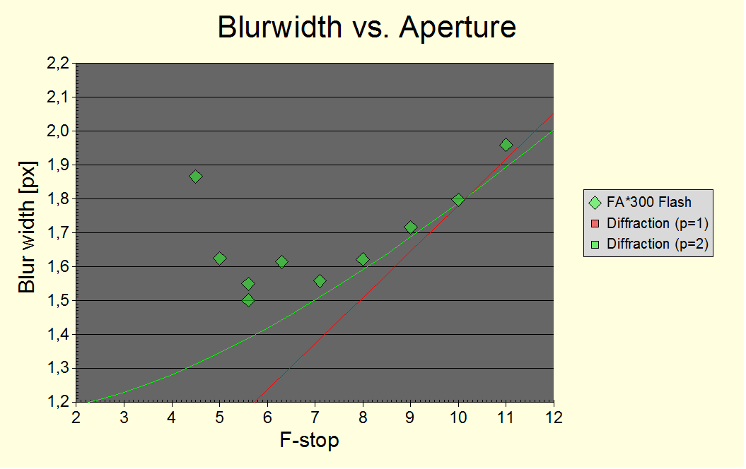
Fig. 8 Dependency of edge blur width with aperture. The blur width as given by the equation above is shown too (with a static blur offset of 1.16 px in the case of the p=2– green line).λ = 550 nm was used. The FA*300 lens is an f/4.5 lens.

The p is the exponent in the Kodak formula used. p=2 yields a more reasonable static blur offset and p=1 turns out to be inapplicable when taking the blur at small N due to aberration and defocus into account.

We will combine blur b_diff due to diffraction using the Kodak formula with exponent p=2. This means it combines like defocus for an otherwise sharp signal.

To summarize: For green light, the Raleigh size f₉ for half a cycle is 0.336 N µm and the f₅₀ blur width is 0.682 N µm for an aperture f-stop N.

2.3. Defocus

Defocus causes (with an ideal lens) a point to be projected as disk with finite diameter coc, the so-called circle of confusion (CoC).

The CoC is an image of the lens' exit pupil projected onto an out-of-focus plane. If this plane is a distance dfapart from the true focal plane (has a focus error df), then the CoC's diameter is

coc = df / N

where N is the lens aperture's f-stop number. Defocus causes additional blur. As above, we will denote the circle of confusion diameter expressed in units of λN by a strikethrough symbol C:

C = coc / (λN) = df / (λN²)

2.3.1. Classical defocus blur and reason for a wave-optical treatment

There is a ray-optical, classical treatment to derive the MTF of a defocused lens. However, as the circle of confusion approaches the size of the Airy disk, the classical treatment produces a large error. The reason can be seen in the following image:

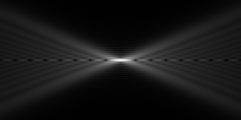
Fig. 9 A slice through the 3-dimensional PSF (point spread function), the image formed when depicting a single bright point, before, at and behind the focus plane.

[from upload.wikimedia.org/wikipedia/commons/1/10/Spherical-aberration-slice.jpg ]

Due to diffraction, the image of a point source in the focal plane becomes the Airy pattern with rings separated by black (cf. above). But by defocussing, the image doesn't simply become fuzzy. The outer rings receive more energy which blurs the image. But the inner ring becomes smaller! The consequence is that very small amounts of defocus do not additionally blur the image! (Defocus is actually scientifically used to reconstruct phase information and additional image resolution.) Eventually, this explains why we treat defocus in a full wave-optical fashion now.

H. H. Hopkins in 1955 published the corresponding original work: "The frequency response of a defocused optical system" [ www.jstor.org/discover/10.2307/99629?uid=3737864&uid=2&uid=4&sid=21100656738486 ] Hopkins laid the foundation for construction of all modern photo lenses and actually invented the zoom lens himself. But his work has, as far as I can see, not yet been made accessible to photographers (it uses terms like wavefront phase errors which isn't something a photographer can refer to). Let me try to change that now.

The MTF of defocus for small enough apertures (sin x ≈ tan x) is:

MTF_defocus= MTF_a / MTF_diff where MTF_a =

and MTF_diff (cf. above) =

expressed in terms of k and C (cf. above). The full MTF for defocus plus diffraction is MTF_a.

In order to make this result more accessible, I show a graph for C = 10. As explained above, at an f-stop of N=1.8 and for a 5 µm pixel, this would correspond to the circle of confusion covering 10 µm or 2 pixels. And it would mark a focus error (shift of focus plane) of 18 µm.

As you can see in  Fig. 10, the frequency k₅₀where MTF becomes 0.5 is roughly k₅₀=Q/(√2 C)with Q ≈ 1. The corresponding blur width is 0.5/k₅₀or:

b_defocus= Q^-1√½ C

i.e., the blur width is 71% the diameter of the circle of confusion, if we ignore Qfor a second. The width where all resolution is killed (zero contrast) is Q^-11.22 C.

So, while the diffraction blur width is 51%of the diameter of the Airydisc, the defocus blur width is 71%the diameter of the circle of confusionwhich is 40% larger.

The same relation holds about true for the vanishing frequency (bandwidth). This is an important result if we want to relate both sources of blur to each other. This consideration is critical but normally missing when deriving the so-called "optimum aperture" ("förderliche Blende" in German). Both diameters are then typically compared directly. There is the added difficulty that the standard deviation of distance from the center diverges for diffraction.

Fig. 10MTF for defocus of C = 10 (without diffraction), e.g., a focus error of 18 µm at an f-stop of 1.8 (red curce). The horizontal axis is k, the vertical axis is the transfer function contrast MTF(k).

The MTF for diffraction is shown too (blue curve). The ray-optical MTF for defocus is ½ (green line) at k₅₀=1/(√2 C)and vanishes at k₀=1.22/C(blue steps). In the graph above, the performance is better due to wave-optical effects but will decrease to the ray-optical values if Cbecomes large enough.

Fig. 11MTF for defocus of C = 1, 2, 3, 5, 10, 20, and 50 (red lines, from above). The horizontal axis is k.

Some notes: The MTF for defocus of C = 3 (3.003 exactly) is roughly equal to the MTF for diffraction up to and at k₅₀. For C ≤ 5, MTF does not become zero! For larger defocus, it approaches the classical MTF for defocus as described in Fig. 10. At C = 3, the CoC is 1.22x larger than the Airy disk! The MTF in Fig. 10 is the 3^rd red curve here, counting from the left.

Additional notes: the full MTF including diffraction is obtained by multiplication with the MTF for diffraction (blue curve). And the MTF for defocus w/o diffraction is symmetrical around k=0.5.

The fact that the MTF becomes negative for large defocus is known as the phenomenon of spurious resolution where line patterns are imaged with a wrong number of lines of weak contrast.

Before we proceed, let me show the MTF for defocus for a setof defocus parameters C(cf. Fig. 11).

The MTF for defocus (w/o diffraction) is symmetrical around k = ½.

As far as I know, this result wasn't published before. It allows to express MTF(k)in terms of MTF(1-k). This is an impportant property because the series expansion for MTF(k)for defocus converges only slowly as k=1is approached but converges rapidly around k=0.

As you can see, the MTF starts to look unlike a classical MTF for defocus for small values of defocus C ≤ 5 (CoC smaller than twice the Airy disk). This is an area large enough to be of interest. It is the area where defocus blur is significantly determined by quantum or wave-optical effects.

2.3.2. Wave-optical effect

In a classical, ray-optical treatment, the defocus blur is expressed as b_defocus= Q^-1√½ C with Q=1.

Let's have a look at the MTF function at the corresponding k = 0.5/b. It should be 50%:

Fig. 12 MTF_defocus(k = 0.5/b_defocus, Q = 1) as a function of C (horizontal axis).

The deviation at C =1is massive but is approaching the ray-optical result (0.5) for large enough values of C . We can cope with this effect in two ways:

1. We modify the Kodak formula by using a matching power coefficient p when combining blur due to diffraction and defocus.

   It turns out that this is doable with good precision using Q=1 and p=2.8.

2. However, we prefer to use the RMS-like Kodak formula with p=2. Obviously, p=1 would be a bad match. We have then computed the values for Q (when entered into the blur term for defocus in the Kodak formula) which best matches the overall blur of diffraction and defocus combined. The heurisic result is (cf. ):

   Q^-1 ≈ 1 – 1 / (3 C)

Fig. 13 The wave-optical or quantum correction factor Q^-1 as a function C between 1 and 10 (blur points).

The red line shows the heuristic approximation curve above which is > 95 % accurate for C ≥ 1.

This particular form has the nice property that it leads to a simple, yet refined version of our blur width for a defocused system:

b_defocus= √½ (C– 1/3) – or which is the same:

b_defocus ≈ 0.71 (coc – N/5.6 [µm])

This is the same formula as above, but now with Q^-1 filled in.

So, the MTF₅₀ blur width for a defocused system is obtained by taking the circle of confusion diameter cocin µm, subtracting ≈N/5.6, and dividing the result by √2.

As far as I know, this result is new (in the photographic community) and easy enough to apply. It takes the wave-optical effects into account. Of course, a negative result is to be replaced by zero as defocus doesn't defeat diffraction. The resulting blur width can be combined with other sources of blur using the Kodak formula with p=2.

2.3.3. Tolerance for defocus

The original paper derives a tolerance for defocus where diffraction MTF is reduced by 20% or less. It is:

C< 0.40 / k

or with f = 0.5/ρ [cy/µm] and k = f λ η :

coc < 0.80 ρ

So, the "surprising" result is that focus errors remain invisible if their circle of confusion remains smaller than a pixel (at coc=ρ, the loss is 32% though). What a break-thru result ;)

2.3.4. Photographic example

We know how defocus blurs an image for a known circle of confusion diameter coc. Now, we need to relate coc to common terms like f-stop and focal distances.

The shift df of the focal plane in the image space can be translated to a shift sof the focal plane in the subject space. Using the thin lens equation, it is:

s = 1 / ((1 + df (b + g) / b²) M²) df ≈ 1/M² df

where M= b / g is the image magnification. And with coc as given in section 2.3 on page 17:

df ≈ s M²

coc ≈ s M² / N

C≈ (s / λ) (M / N)²

By combining with the formula for defocus blur above we obtain:

b_defocus= √½ (s M²/ N – N / 5.6)
where s is the focus shift in the real space,
M the image magnification and Nthe f-stop.

Fig. 14 shows the change of blur due to defocus in a real-world experiment. It turns out that the theoretical result is in nice coincidence with the theory (formula above) if the Kodak formula (p=2) is applied to unsharpened blur measurements. Obviously, sharpening kills part of the defocus blur too. So, this is how overall blur for sharpened images was eventually computed (cf. section 2.1 for b_soft):

b(s) = √[(b(0) + b_soft)²+ b_defocus(s)²] – b_soft

The red line in Fig. 14 shows the expected blur values according to the formula above. The green line connects actual edge blur measurements, with no offset and expressed in px.

Fig. 14 The variation of edge blur width b with amount of defocus by varying (shifting) the subject distance. The official parameters are: lens focal length f=250mm, subject distance g=4700mm, aperture N=5.6, shift s is the x axis and pixel size ρ=5µm.

However, a zoom lens close focused to a target can have largely different parameters (the ones mentioned above produce large deviations, up to a factor two!). I measured the magnification M directly (which correponds to f=191 mm) and corrected the effective aperture f-stop using the thin lens formula (at this focus distance, it is f/5.9).

The shift is the amount of defocus in the subject space, with negative values corresponding to backfocus. The red line is the theoretical curve as discussed above. The green line is the edge blur as measured.

The 0.8 ρ focus tolerance expressed above corresponds to |s| < 14 mm. Interestingly, the green measured values seem to be a tad more sensitive for true focus. But it may be accidental. The 14 mm tolerance requires a 23 µm accuracy in the focal plane (in this example).

The tolerance region in the figure above (14 mm) is the depth of field for pixels remaining sharp. This differs from the photographic depth of field (DoF). There are enough treatments of the photographic DoF due to acceptable defocus, e.g., by applying the Zeiss formula that cocshould stay smaller than 1/1730 of the image diagonal, typically chosen on 35mm film to be 25 µm (1/1730) or 0.03mm (1/1500).

With the Zeiss CoC parameter for an APSC camera (17 µm) the classical DoF formula yields a DoF of ±56 mm. So, the tolerable "pixel peep" shift is about ¼ of the DoF.

2.3.5. A note on equivalency

The image magnification is squared in the formula for dfin the previous section 2.3.4. This means that a sensor of e.g., half size requires four times the focus accuracy df^-1for equivalent results (i.e., same shift sin subject space). Moreover, a sensor of half size would then typically use a phase AF measurement triangle base of only half size too (e.g. because it uses an AF sensor of same f-stop) actually lowering focus accuracy (by half) rather than increasingit. So, both effects combined mean that the technical challenges for accurate focus for a sensor of half size are 8x harder.

However, M/N (and C) are sensor-size independent for equivalent lenses and the same focus accuracy. Nevertheless, if the lower focus accuracy is offset by using (non-equivalent) lenses of constant f-stop, C will decrease and behave more ray-optically.

I consider the dramatic (square or cubic) improvement of focus accuracy with sensor size to be themain advantage of a larger sensor size as it can't be offset by use of equivalent lenses.

2.3.6. Ability of deconvolution operators to reduce defocus blur

... in progress

The previous section on the possible cancellation of the BAA filter and the reduction of perceived defocus blur due to sharpening contained some information already. It works well as long as the blur width must not be reduced by more than 2 pixels and as long as image noise is very small.

However, blur due to defocus can be removed for much larger blur widths. This is possible because the blur kernel is known and can be algorithmically inverted. However, the corresponding mathematical operator is instable, i.e., small input errors (e.g., noise or a deviation in the point spread function) cause large output errors (e.g., artefacts). This is why "regularization" is required for pleasing results. On the other hand, this regularization reduces the output sharpness.

I tried a number of algorithms and products, incl. Topaz Infocus. But only FocusMagic could convince me. FocusMagic successfully restores image sharpness for defocus blur up to 10 pixels. Sometimes more. But I would then recommend to first reduce the image size. By restoring image sharpness, I mean restoring image detail. You'll see information which was invisible beforehand.

Unfortunately, FocusMagic is 32 bit software and has trouble to run on more recent machines. It hasn't seen an update for a long time. Still, it seems to be by far the best option out there.

… an article update will show side be side comparisons with USM, LR and Infocus sharpening.

2.4. Lens aberrations

2.4.1. Defocus, Spherical aberration, Coma, Astigmatism

... in progress

cf. http://www.telescope-optics.net/mtf.htm and http://demonstrations.wolfram.com/SeidelOpticalAberrations/

Also, cf. the page MTF3 in the 1^st link on aberration compounding: they use the Kodak formula with p=2.

2.5. Shake

Shake originates from a change of the optical axis angles (nick, yaw and rotation) during the exposure. As magnification grows towards M=1, a change of the optical axis translational parameters (positional shift) starts to play a rôle as well. We don't discuss shake in macro photography. In general, preventing it is as challenging as in astro photography.

2.5.1. Measuring shake

Normal shake is most easily measured by taking test shots of a slanted edge test chart (cf. Fig. 4 on p. 7). Translational shake can be ignored for g>100 f, e.g., if the chart for a 50 mm lens test is on a wall 5 m away. The same camera displacement then leads to only ≈1% blur if translational when compared to rotational, e.g., a 5 px blur measure has less than 0.1 px translational error. This is also less than a "four stop" blur reduction (≈6%) due to some image stabilization or shake reduction apparatus.

For free-hand test shots, care must be taken to stay within a region of neglegible blur due to defocus. Use the formula in section 2.3 Defocus on p. 17 to estimate the region and make sure it spans 100 mm at least. When manual-focussing using LiveView, make sure you still hold the camera viewfinder at your eye. Using contrast AF may be your only choice then...

The blur due to shake b_shake is combined using the Kodak formula with p=2.

Therefore, an accurate estimation of b_shake requires an accurate knowledge of the static blur without shake. Unfortunately, tripod measurements aren't normally accurate enough. You either need as many tripod measurements as free-hand ones, or you use an extrapolated blur value at zero exposure time to become the offset value. Note however, that the extrapolation method is only valid if you don't change aperture or ISO, i.e., if you use an adjustable artificial source of light. Also note that most tripods aren't stable enough for short time shake measurements (even with mirror lockup and remote triggering) and the camera clamped directly to a massive rock table or alike may be the better choice.

2.5.1.1. The double slanted squares method

It can be shown that the amount of motion blur in an individual image due to angular velocity can be measured in a self-contained manner using a test chart made of two slanted squares, tilted at 22.5° and -22.5°, resp. against the horizon. Be:

a_1,2 = b²₂ - b²₁(widths of a vertical and horizontal edge at the first square), and
a_3,4 = b²₄ - b²₃(widths of a vertical and horizontal edge at the second square), then

b_shake = (a²_1,2 + a²_3,4)^¼(the exponent is ¼ if too tiny to read)

b²₀ = (b²₁ + b²₂ + b²₃ + b²₄) / 4 - b²_shake/2

φ= - arccot ((a_3,4 – a_1,2) / (a_3,4 + a_1,2)) / 2

independendly from the direction φof shake. This method should be combined with averaging the edge blur widths b²_i of both parallel edges for every square, i.e., 8 edge widths should be computed. It is therefore important to make sure that lens aberrations are constant throughout the entire range covered by the two squares.

The averaging of parallel edges with opposite dark/bright transitions is required because the non-linearity of the luminosity response curve (after sharpening) makes the edge blur measure become dependent on the sign of direction of shake.

b_shake and b₀ as measured by this method do already separate the blur due to shake and the static offset at the level of a single test chart image.

Note: This method of double squares and 8 edges and formula is my discovery. The publication in this paper makes it "prior art" for any forthcoming patent application. The method includes using double slanted squares in the absence of shake in order to separately measure different kinds of aberration.

2.5.1.2. The normal slanted edge method

The normal slanted edge method measures 1, 2 or 4 edges in the slanted edge chart. Two edges may be measured to separate the blur in nick and in yaw direction from each other. This gives an idea about the approximate direction φ of blur. Four edges (with two edges parallel) are measured to minimize the effect of a non-linear luminosity response curve as dicussed above.

It turns out that about 20 measurements are required for acceptable variations; and about 10 tripod measurements for the static offset taken at identical shooting parameters. The Kodak formula is applicable to mean values rather than individual values and requires knowledge of the static blur offset. The total mean blur may then be estimated by

b²_shake= b²_nick + b²_yaw-2 b²₀ or
b²_shake= 2 (b²- b²₀)

in the absence of two measured orthogonal edges per test chart.

2.5.2. Expected shake

The nice thing about b_shake is its direct correlation to the angular movement of the camera during the exposure,

b_shake (t) = υ t f

where υis the angular velocity (rad/s) of camera shake, t is the exposure time and f is the focal length. Of course, this only applies if tis small compared against the periodicity of shake oscillations.

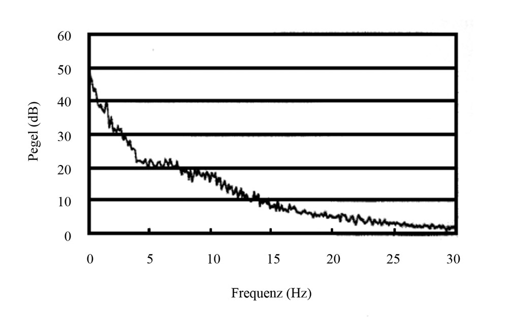The chart to the right shows the power distribution of free-hand shake for a typical human photographer [Source: http://www.colorfoto.deby Boris Golik]. It looks
a lot like 1/f noise but with a peak around 4 - 10 Hz. For a single frequency of shake (i.e., for a harmonic shake), I computed the blur width to be

b²_shake (t) = ~ f ² (½ – (cos(ω t) – 1) / (ω t)²) where ω = 2 π frequency_shake

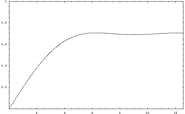The plot to the right shows this harmonic blur as a function of exposure time t (in some arbitrary units).

In the general case of 1/f noise though, in particular in the form of 1/f ^q noise for some exponent q, the blur becomes

b_shake (t) = ~ f t^{(q – 1)}

and for q=2, we get a linear form for arbitrary exposure times. In general with an emphasis on some shake frequency, we may expect a superposition of a clipped linear law and a power law for some exponent.

A shake reduction mechanism (either optically by lens shift or mechanically by sensor shift) will almost certainly correctly register the dominant harmonic part (their gyro angular velocity sensors typically are fast enough for frequencies up to 20 Hz) and reduce the corresponding amplitude of shake by some factor. Factors in the vicinity of a tenth are common. The 1/f noise parts may be reduced less, esp. their higher frequency terms. This can lead to a different exponent when fitting the b_shake (t) function.

2.5.3. Empirical results

The following is a chart of real measurements shake b_shake(t)/f due to free-hand vibration and other sources like shutter, mirror slap etc.

Inserting a known pixel size and dividing by the focal length f, b_shake(t)/f becomes a dimensionless function, i.e., a blur width best measured in mrad (1 mrad ≈1 / 17.5°). For freehand photography without using image stabilization technology, this function should only depend on the photographer and weight (moment of inertia) of the camera+lens.

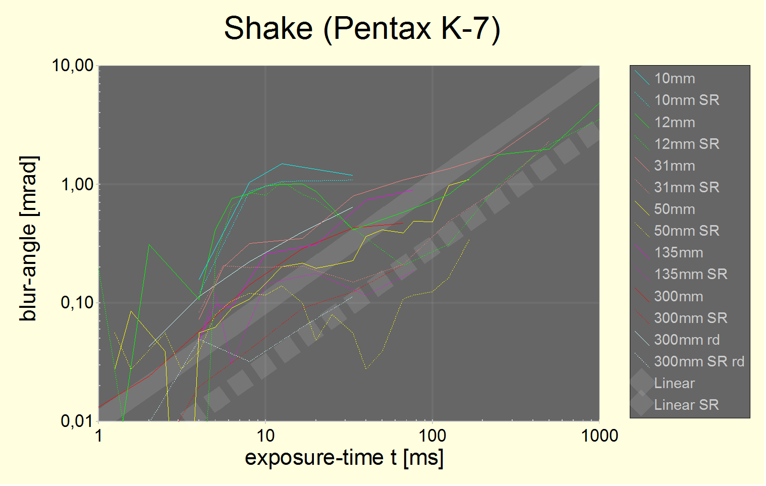
Fig. 15 Image shake as measured with a Pentax K-7. The K-7 has 5µm pixels. The wide straight lines are linear fits with a constant angular velocity of υ=10 mrad/sand 3 mrad/swith Pentax shake reduction (SR) disabled and enabled, respectively.

For all but the largest focal lengths, blur angles smaller than 0.1 mrad are not measurable. For the largest focal lenghts (135 mm and most of all, 300 mm) one may see however that the linear fit extends down to about 1 ms. It applies nicely above 30 ms as well. The region between 4 ms and 30 ms is specific to a particular camera model and may include shake due to shutter motion.

The data in this chart are collected from 4 testers, 4 camera bodies and 7 different lenses. It may be one of the most complete charts of its kind. In this log-log plot, a linear fit (as described by the first formula in section 2.5.2) always looks like a straight line of slope +1. Different factors lead to parallel lines with their distance being their relative ratio of factors. The SR line corresponds to a constant benefit of 1.7 f-stops. Some combinations of focal length and exposure time beat that, others don't.

So, our empirical result is that a linear relationship of blur and exposure time is an acceptably good relationship with υ≈10 mrad/sfor free hand exposures and υ≈1-5 mrad/sfor various image stabilization techniques and situations.

To translate this to a blur width, just multiply with focal length, exposure time, 1/pixel size. E.g.:

b_SR (t=1/15s,f=50mm,u=5µm)= 3/1000 * 1/15 * 50mm / 0.005mm = 2 px

This width must then be added using the Kodak formula using p=2, increasing a perfect pixel's blur from 1.25 px to 2.35 px or by ≈100%. Note that in this particular example, the Pentax K-7 actually performs better. The formula given shall serve as rule of thumb only in an attempt to provide a more precise version of the famous 35 mm 1/f rule for taking shake-free photos.

2.5.4. Tripod classification

One well known image stabilization technology is the tripod which shall eliminate blur from free hand shake and other sources of shake. We found that simply referring to a "tripod" is not good enough. So, we use the following classification of tripods:

• Class A: A tripod which is very massive (like 100 kg) and has zero slackness in the junction to the camera. An example is a camera clamped to a massive stone table. Or an equivalent tripod.

• Class B: A tripod which damps normal vibrations by several order of magnitudes if given some relaxation time. An example is the normal steel spike tripod sitting on a concrete surface. Class B requires specification of a relaxation time.

• Class C: A tripod which can maintain a constant direction of view (which is no source of shake) but would not resist to short impacts of force which then may change its direction. Class C requires specification of a mass.

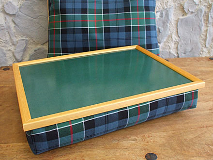
  Another example is a Scottish laptray when used upside down (flat side down) on a concrete surface. It is filled with little balls made of polystyrene and will keep its form. It is an excellent zero mass class C tripod. It behaves like a hand without inducing hand shake.

  

• Class D: A camera placed on a stable table without fixing it.

• Class E: A monopod with a single rod only.

Additionally, testing should use mirror lockup and remote triggering when applicable or be specified otherwise.

2.6. Motion blur

... in progress

2.7. Noise

... in progress

Taking slanted edge test chart shots at higher ISO actually leads to artificially reduced edge blur measurements even though the true resolving power at higher ISO is less. This is due to a loss of tonal detail at higher ISO which acts like higher contrast or stronger sharpening. This effect is about as strong as the diffraction effect and acts in the opposite direction (if ISO is increased to compensate for a larger f-stop).

2.8. Atmospheric perturbations

... in progress

cf. http://blog.falklumo.com/2010/04/howto-long-range-telephoto-shots.html

2.9. Precision and calibration

... in progress

3. Practical considerations and examples

... in progress