Nikon D800 AA filter vs. D800E
– Whitepaper –
Falk Lumo [LumoLabs (fl)]
Dieter Lukas [panobilder.de]
|
Version: |
May 9, 2012, v1.0 |
|
Status: |
Final |
|
Print version: |
|
|
Publication URL: |
|
|
Public comments: |
|
|
Deutsche Fassung: |
This white paper publishes a full laboratory measurement of the Nikon D800's Bayer-AA filter and provides a short discussion in terms of differences between a D800 and D800E.
1. Introduction
Nikon decided to make two versions of its Nikon D800 full frame SLR camera which is in so high demand everywhere.
One with a Bayer-AA filter (the D800) and one without (the D800E). Obviously, the D800 is meant for APS-C and 35mm full frame SLR crossgraders as all current such cameras with a Bayer sensor have a Bayer-AA filter. While the D800E is meant for medium format (or Leica M9) crossgraders as all current such cameras have no Bayer-AA filter. The latter makes sense because of the high resolution of the D800/E which at 36 MP touches what once was medium format territory (40 MP).
Don't believe for a second that Nikon created the two versions for technical reasons. They have not. They created two versions to serve two separate markets. It is this simple. So, don't expect Nikon has any clue what camera would be the better one for you. All they'll try is ask you questions to figure out which market you belong to. Not their business, not really helping in your decision.
If you want to know what's really in the boxes and how it really differs, here you may find it. We may have done the hard work for you.
2. Background
First and foremost, what everybody calls "AA filter" or "anti-aliasing filter" or "low-pass filter" isn't one. A low pass filter destroys the signal at high spatial frequencies. Every digital camera does have a low pass filter. But it is the finite photo-sensitive size of a sensel or pixel, typically enlarged to almost the full sensel's extensions by a microlens. The microlens array provides a better quantum efficiency (less photons get lost) but also provides a camera's true low pass filter. Assuming a fill factor of 100%, it destroys signal at twice the Nyquist frequency (the spatial frequency which sensels are placed at on the sensor) and dampens signal at the Nyquist frequency to 64%.
Please, refer to the whitepaper "Understanding Image Sharpness" at LumoLabs for further detail.
The problem is as follows: Assume a ray (e.g., from a star) reaches your camera and hits a single sensel. Above the sensel will be a green, red or blue filter from the Bayer filter array. This means that the camera will see a green, red or blue star. There is no way for the camera to detect the star's real color, and no smart software can recover the missing color information. This is the false color problem when demosaicing specular highlights ("stars") or contrast edges. If contrast edges form a regular pattern, the false color will vary slowly across the image forming what is called a false color moiré pattern (looking like a rainbow artefact, cf. Fig. 1).
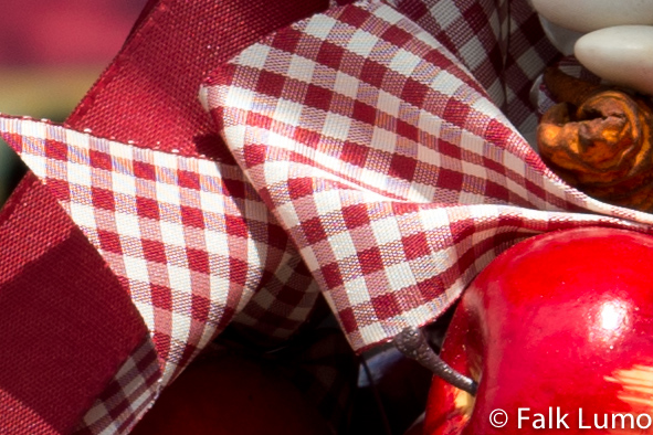
Fig. 1 1:1 crop (8% of original dimensions) of a photo taken with my Nikon D800E. The image shows some false color moiré in the red/white fabric pattern. Both Nikon CNX2 and Adobe Lightroom 4 would be able to remove this artefact. It hasn't applied here on purpose. Photo shot outdoor and hand-held/AF.
Note you'll have to search hard to find examples in real photographs. There aren't many examples yet on the internet, many famous photographers report to be "still searching" …
Of course, the entire problem disappears if a ray hits more then a single sensel. Because then the color can be reconstructed by comparing the signal from neighboring sensels having different Bayer filter colors.
This is what a filter achieves which I call the "Bayer-AA filter". It actually isn't a low pass filter at all. It typically is a pair of lithium niobate crystal plates turned 90° with respect to each other. Lithium niobate is birefringent and splits a ray into two. The pair therefore splits a ray into four, designed to hit exactly one of each of the four Bayer color filters. In order to achieve this goal, the ray split distance must be equal to the sensel pitch (or pixel size). The result is exact color reproduction. Such a Bayer-AA filter is called to have 100% strength.
But the birefringent crystals interact with the microlens array and combine to a low pass filter of only half the spatial frequency: Now, the signal at the Nyquist frequency itself is destroyed. Because vendors don't want to sacrifice the full sensor resolution, they typically design their Bayer-AA filters to be weaker where a 0% strength would correspond to their absence.
The Nikon D800E has such a 0% strength. However, it isn't achieved by replacing the birefringent crystals. This would require a re-calibration of the optical path, AF module, focus screen and color profiles. Rather, Nikon uses a pair of lithium niobate crystal plates turned 180° with respect to each other which happen to cancel each other (if aligned properly).
By comparing the D800E and D800, we are going to derive the exact strength of the Bayer-AA filter in the D800. You most likely won't find such a result anywhere else on the internet.
3. Setting up the experiment
In order to arrive to our goal, we have to measure each camera's modulation transfer function (MTF) as precisely as possible. Again, please refer to the whitepaper "Understanding Image Sharpness" at LumoLabs to understand what it means.
The idea is as follows: Once we have the MTF for the D800 and the one for the D800E, their quotient MTFD800(f)/MTFD800E(f) will provide an MTFBAA(f) which describes the effect of the Bayer-AA (BAA) filter in the D800:
MTFD800(f) = MTFBAA(f) ×MTFD800E(f)
From MTFBAA, we'll be able to derive the physical properties of the Bayer-AA filter Nikon built into the D800.
Unfortunately, almost every author of web tests fails to measure MTFs precisely enough to isolate individual effects. Not only must illumination, motion blur, shake, lens blur etc. be constant across measurements. But especially focus must be aquired with the exact same accuracy. And we're talking a few µm here! It turns out that autofocus, contrast detect autofocus, zoomed liveview manual focus and even the typical focus series are not accurate enough.
In order to control most variables, we used the identical lens, a Nikkor 24-70/2.8G, at 50mm f/4.0 in the center, using mirror lockup, remote trigger, studio flash to control illumination, motion blur and shake. The distance was 2.5 m (50x focal length).
3.1. Controlling focus
In order to control focus, we did a focus bracketing series using a focusing rail slider using controlled increments (9 mm) as derived from the LumoLabs work on the defocus MTF.
In Fig. 2, you find the quality of focus varying with the position within the focus bracket.
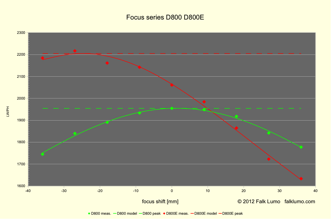
Fig. 2 Effective resolution as a function of focus shift in the subject space.
Resolution is expressed as inverse 10-90% edge rise width, where images are developed by Lightroom PV2010 with all sliders flat (no brightness, contrast, sharpening).
Shift is expressed in subject space (a negative shift is nearer to the subject), where shift 0 identifies the position corresponding to contrast detect autofocus.
The red line corresponds to the D800E, green D800. The lines are following the mathematical model for defocus blur and the dashed lines are the exact best resolution figures derived from fitting the entire focus bracketing series, i.e., not requiring hitting the exact point.
The derived exact in-focus resolutions are 1955 LW/PH (D800) and 2205 LW/PH (D800E). The best available test shots (0 mm D800; -27 mm D800E) have a deviation of 0.5 % or less from that value. This was deemed good enough for our purpose. Note that a visual inspection in order to select the best shot wouldn't be possible with such tiny differences. They are invisible to the naked eye.
4. Test shots and MTFs
DSC_0746.tif (D800) (not all browsers show the above image)
D800 (if reading in a browser, then please open images in a separate tab, or download the TIFF files)
DSC_0192.tif (D800E) (not all browsers show the above image)
D800E
Fig. 3 Largely magnified inner crop of the selected test shots. Refer to later discussion about how sharpened and properly treated samples look like.
You may note a slight difference in scale. It is due to a little accident: we didn't tape the zoom ring and the D800E images are at 48 mm rather than at 50 mm. However, due to the scale-invariant method of MTF computation and lens performance which should vary by only 0.3% here, this should have no measurable impact on results.
We use a modified version of the ISO 12233 test chart, one that uses 4x magnified tiles and we also didn't fill the frame on purpose. As a result, the Nyquist frequency is at the spatial frequency marked by the figure "6" in magnified tiles ("24" in normal size parts, not visible in the crops above).
Using the slanted edge method, we derive the respective MTFs as follows (cf. Fig. 4).
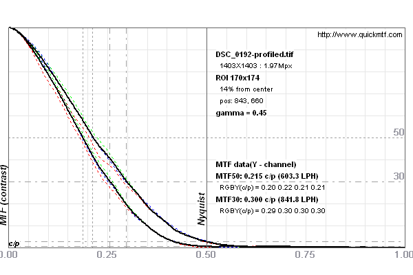
Fig. 4 MTF of the Nikon D800 (lower curve) and D800E (upper curve).
Result for unsharpened but profile-corrected images. At the Nyquist frequency, the MTF for the D800 does not entirely vanish. This is the prerequisite to be able to recover detail at the Nyquist frequency via sharpening (cf. below). The corresponding contrast values at the Nyquist frequency are ~0.5% and ~2.5% resp.
Note that lens profile correction like scaling or rotation involves a resampling of pixels lowering the contrast near the Nyquist frequency. This is avoidable. However, in our context of comparing the two cameras, it delivers a more stable end result. Other MTFs leaving more contrast near the Nyquist frequency are discussed below.
From Fig. 4, we can derive MTFBAA (cf. Fig. 5). We compare this measured MTF function with a theoretical prediction we can provide.
We have discussed above that both, the D800 and D800E have low pass filters (after taking the micro lens array into account) where the difference lies in the fact that the low pass cut-off frequency differs (after taking the Bayer-AA filter into account).
Using
sinc(x) := sin(x) / x
we predict
MTFBAA (f) = sinc ((1+σ) π f) / sinc (π f)
whereσ is the Bayer-AA filter strength (as discussed above), ranging from 0 to 1, or 0 % to 100 %.
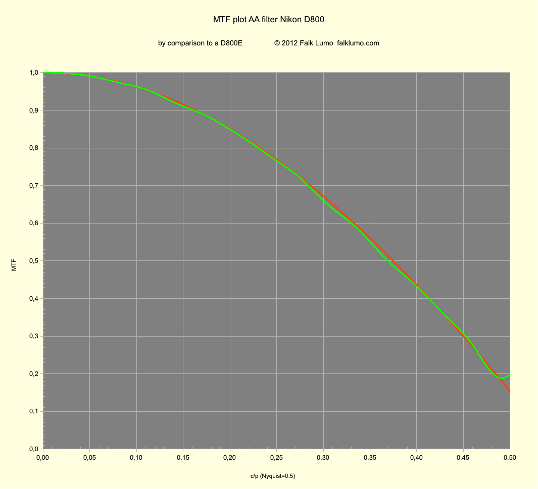
Fig. 5 MTFBAA(f) for the Bayer-AA filter component alone (green line measured).
The red line is the function as theoretically predicted for a fitted Bayer-AA filter strength of σ = 0.82.
As you can see in Fig. 5, the measured MTF curve matches the prediction using σ = 0.82 excellently. However, if we use unsharpened images without profile correction, we obtain somewhat less stable results, matching the prediction only below 0.35 c/p with a corresponding value of σ = ~0.67.
Overall, we conclude that
The computed Bayer-AA filter strength of the D800 is 75% ± 7%.
The corresponding birefringent ray split distance is 3.3 µm – 4.0 µm.
The ray split distance should be verified by an independent measurement on an optical bench.
5. Practical consideration
A Bayer-AA filter strength of ~75% is moderate. In an ideal situation (low ISO, sharp lens, no shake, good focus etc.) it leaves enough contrast at the Nyquist frequency to recover all detail a sensor with the same resolution but without a Bayer-AA filter could have captured. On the other hand, it cannot completely eliminate the risk of false color moiré, only reduce its likelihood and visibility.
An even weaker Bayer-AA filter strength of maybe ~50% would leave too much contrast at the Nyquist frequency and the impact on false color moiré would have been small only.
In order to discuss the usability of fine detail with both cameras, we'll first compare the MTF50 resolution figures we obtain from either camera using different sharpening parameters.
5.1. Sharpening parameter landscape
The most important single factor determining any digital MTF50 measurement is … sharpening!
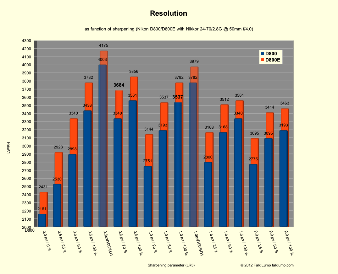
Fig. 6 Various values for MTF50 resolution for a perfect test shot using a D800 or D800E.
The images are rendered using Lightroom PV2010 with standard parameters except for sharpening. This setting already increases contrast and resolution above a flat rendering, even for zero sharpening.
All other sharpening parameters are as labelled. The detail slider was at its standard value (25%) except for the "D1" labels where it was at 100%. Because this involves deconvolution, I marked the corresponding bars with light transparancy. For best results, the D800E would require deconvolution with less than 0.5 px radius, something Lightroom does not offer.
If one is oversharpening, the corresponding MTF looks odd and resolution figures begin to drop. An extreme example is given in Fig. 7.
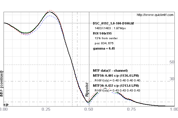
Fig. 7 MTF for an oversharpened D800E image (radius 1.0 px, 100%, detail 100%). The MTF at Nyquist is almost destroyed and the image exhibits sharpening artefacts.
In Fig. 3, one could compare two 1:1 crops at equal sharpening (i.e., with no sharpening). Now, we select two sharpening settings which we deem to provide appropriate sharpening levels for either camera:
-
D800: 1.0 px radius, 100 % yielding 3537 LW/PH resolution (MTF50).
-
D800E: 0.8 px radius, 70 % yielding 3684 LW/PH resolution (MTF50).
The 4% difference in MTF50 is neglegible. Fig. 8 shows the respective MTF curves. From the sharpening parameter landscape plot above we think that this pair allows for the best peer to peer comparison.
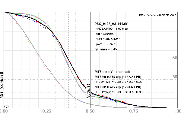
Fig. 8 MTF curves for (differently) sharpened images from D800 and D800E. The black curve is for the sharpened D800E, the grey curves are unsharpened and (differently) sharpened D800 curves. Both curves have equal MTF75.
A 100% (or 1:1) crop from both test chart shots is shown in Fig. 9 and Fig. 10. When browsing the web version, please open images in separate tabs.
It is of course unfortunate that both images don't have exactly equal scale. The differences are marginal though. The D800E crop may exhibit just a tiny bit less traces of sharpening. And it definitely has more false color around the Nyquist frequency patterns. The difference however isn't as striking as one could have assumed: Without a direct peer to peer comparison, it would not be possible to tell the crops apart. i.e., the D800 crops exhibit their fair share of false color as well.
In direct comparison, I'd say the false colors from the D800 maybe have half the saturation of the false colors from the D800E. Overall, all factors considered, I'd say that the ISO test chart is reproduced slightly better by the D800.
A side note: Comparing unsharpened flat images from the D800 and D800E, the 10–90% edge rise width is about 0.3 px less for the D800E. With equally sharpened (0.5 px, 100%) default-processed images, this reduces to about 0.15 px difference. However, the D800 images require about 0.5 px more sharpening radius (i.e., 1.0 px rather than 0.5 px at 100%) to deliver a comparable edge blur width (which in the samples above then is about 1.32 px from both D800 and D800E – an ideal value). We'll refer to this result as "the E being 0.5 px sharper". It is a bit misleading but we explained what we mean. In the comparison shown in Fig. 10, we'll show the result of sharpening the D800E with 0.8 px radius, 70 % amount though (the edge blur width is the same, 0.30 px). Because 0.5 px radius, 100% amount makes the D800E have an even higher MTF50 value.
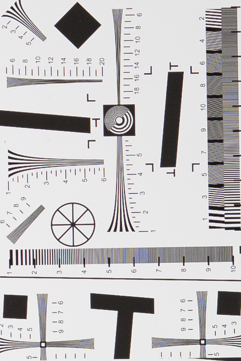
Fig. 9 1:1 (100%) crop of the sharpened D800 test shot.
The Nyquist limit is at line frequencies denoted by "6".
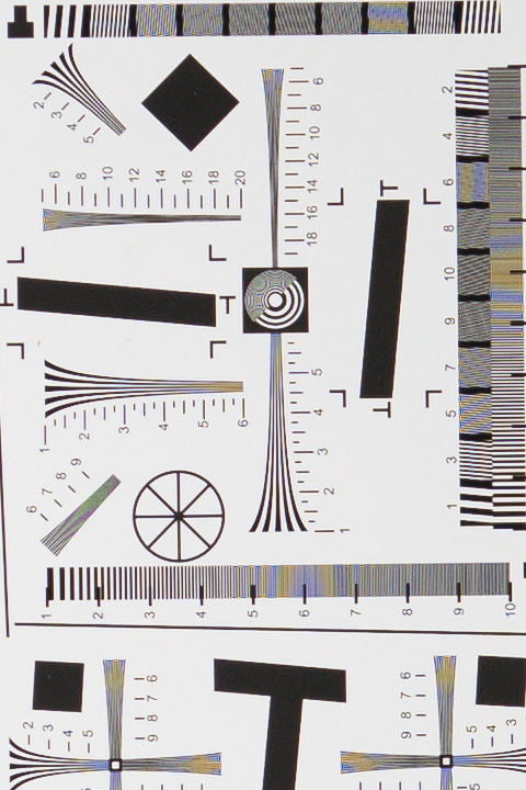
Fig. 10 1:1 (100%) crop of the sharpened D800E test shot.
So, there is an interesting lesson here: In ideal situations where sharpness is maximized, both cameras (D800 and D800E) should show the same false color moiré patterns, only the ones from the D800E should have more striking colors (less muted).
Of course, in less than ideal situations, other sources of blur add to the D800's moderate Bayer-AA filter and completely eliminate the cause of false color moiré while the D800E may still exhibit some.
And in even worse situations, blur would be enough to completely eliminate the cause of false color for the D800E too.
The paradox truth is: in controlled environments with ample of light (studio etc.) and with man-made patterns, the chance to produce a moiré pattern is maximized and the D800 images should offer enough headroom for sharpening to the same level of micro contrast without the same risk of false color moiré. On the other hand, in less controlled environments, the D800E should produce better results because there would be enough other sources of blur. It is paradox because the market segmentation anticipated by Nikon is the opposite (where medium format shooters aka studio shall be more likely to get the D800E).
6. Conclusion
We determined the Bayer-AA filter in the Nikon D800 to be rather weak, around 75% of a full strength filter.
As a consequence, the difference between a D800 and D800E isn't as large as one may think: in a controlled environment, the D800 images can be sharpened to the level of the D800E. The downside is that it can produce some false colors too, although less likely and to a lesser extent.
As a rule of thumb, we found that (assuming 100% amount, in Lightroom terms) subtracting about 0.5 px from the sharpening radius used for a D800 image produces comparable sharpness and acceptable results. In practice, one may of course combine this with a larger radius and lower amount etc. We summarize this into the following headline:
D800: E = 0.5px sharper
Meaning, that with ~100% amount sharpening, the D800E should deliver comparable results with ~0.5 pixels less sharpening radius, compared to a D800. This also means that one should not refrain from sharpening when using the D800E. Just use weaker settings.
As a final note, let me say that it really does not matter so much: The 36 MP of the D800 means that the full pixel quality does not matter anymore in 95% of cases. So, for the most part, the differences between a D800 and D800E can probably be ignored.