Shutter induced blur with the Pentax K-7 camera
– White Paper –
LumoLabs (fl)
(Falk Lumo)
Rüdiger
(Rüdiger at digitalfotonetz.de forum)
Henning
(Henning at digitalfotonetz.de forum)
|
Version: |
1.0.1 of Jul 22, 2010 |
|
Status: |
Final |
|
Print version: |
www.falklumo.com/lumolabs/articles/k7shutter/ShutterBlur. pdf |
|
Publication URL: |
|
|
Public comments |
http://blog.falklumo.com/2010/07/lumolabs-shutter-induced-blur-with-slr.html |
This paper studies the impact of the shutter on image sharpness. The operation of a mechanical shutter is known to have a negative impact on image sharpness. This is old wisdom. However, the exact magnitude of the effect and the question if it is significant in day to day usage is not very well understood. Therefore, we decided to study this effect in detail for the Pentax K-7 digital SLR camera. Of course, we combine this with a study of the (lack of) impact of mirror slap and hand-held operation. We verify the existance of extraneous blur and identify its exact nature and cause. It helps to understand the mechanism leading to this kind of blur and to effectively work around them. All content in this paper is © 2010 authors and coauthors.
A first reading of LumoLabs' white paper „Understanding Image Sharpness“ is highly recommended [www.falklumo.com/lumolabs/articles/sharpness/].
1. Motivation
Internet forums are full of speculation whether there are some inexpected sources of blur for various cameras from several vendors. This paper will stay away from all the fuzz and stick to facts only. Nevertheless, it is good practice to start off with examples, so here we go.
1. 1. An informal example of extraneous blur
Supposed you are the lucky owner of a Pentax K-7 camera and a wide angle lens, then it is actually quite simple to verify for yourself that the effect addressed in this academic paper is a true effect relevant to the real life of a photographer. The effect itself really isn't academic at all. Please, just invest 10 minutes to do a short test. You may be surprised about the outcome and will have learned something in consequence.
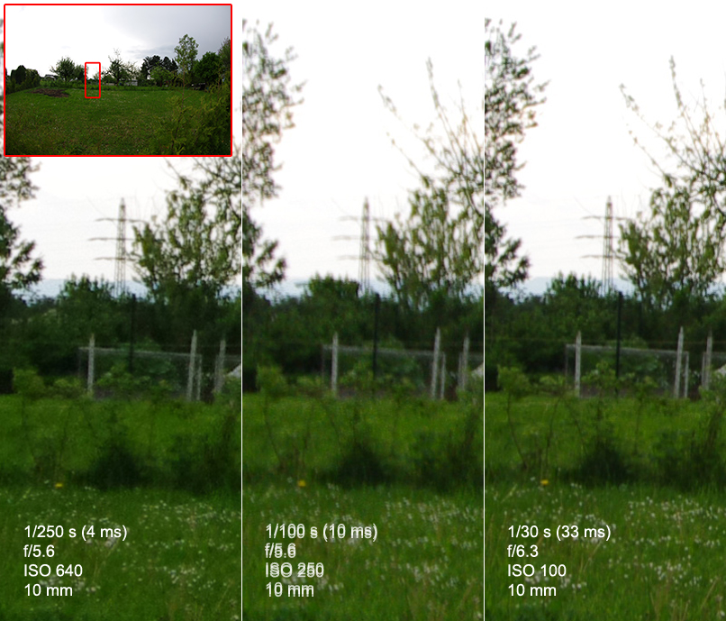
Fig. 1 At the dandelion flowers in the foreground or the electrical tower in the background, you see that the middle image suffers from motion-like blur. Exposure time used was 1/100 s and the blur effect is even more pronounced at 1/80 s as we are going to show. Photos done with a Pentax DA 10-17.
The three crops are 5.7% x 22.2% large crops (processed as 100% crops), cf. inset in the upper left.
The blur in the caption of the middle image is a joke. But it's size (3 px) would be about correct.
We recommend to use a sharp wide angle lens with your K-7 (e.g. DA 4/12-24, DA* 2.8/16-50) or to stop down enough to get sharp images in the center. Also, please do manual focus your lens as autofocus (AF) isn't always giving best results with super wide angle lenses pointed at a distant subject. Then photograph the same scene at the shortest focal length with an exposure time of 1/80 s and 1/25 s, five shots each. You may want to shoot a few different scenes or to make sure that you have a high contrast horizontal structure in your image like a roof top, a window frame at some distance or text. You can use shake reduction (SR) because as we are going to show, the extraneous blur is independent from shake reduction. Of course if not shooting at really short focal lengths like 12 mm, then activating SR helps minimize the normal free hand blur.
Next, examine the image sharpness. If you use the Pentax Digital Camera Utility you can easily compare them in 100% mode. You'll see a thing similiar to fig. .
We predict you to see sharp 1/25 s pictures (if you didn't blow it), but that the 1/80 s images will look fuzzy, almost like being affected from motion blur.
If you repeated the test at 1/250 s, you'll find sharp images again. And if you did the same test with a Pentax K10D or K20D camera then the difference of image sharpness would be much smaller. Therefore, the effect of shutter-induced blur is dependend on the exact model of the camera used as well. The effect is particularly large for the Pentax K-7 camera. However, we did not study the Pentax K-x.
Of course, that the blur is indeed (in)directly triggered by shutter operation is not self-evident. Therefore, we will provide evidence for this in section 4. Testing for alternative causes on p. 12.
1. 2. A more formal example of extraneous blur
The following example of a test chart image with black and white areas (cf. fig. on p. ) is used to actually measure the blur. We use the slanted edge method to measure the blur in up-down (pitch) direction and left-right (yaw) direction independently from each other. We are thus obtaining exact measures for the blur amount and direction.
From our free hand blur formula, it is clear that at 12 mm we should expect blur to be smaller than:
bshake < 10 mrad/s /1000*1/80s*12mm/0.005 (mm/px) = 0.3 px
In the sample below, the blur from the 10-90% edge rise width in the yaw-direction is 1.48 px and in line with this expectation indeed. So, we don't see an example of defocussing and a decentering defect was excluded by other tests. Simple hand shake is unlikely and further excluded by the fact that a type-C tripod was used. Moreover, a hand shake blur's LSF is not normally double-peaked.
At least 10 measures (sometimes up to 200) are then used to compute mean values with an acceptable error margin. The „sharpness“ white paper explains all of this in more detail. Unforunately, all charts in this report are without error bars (but errors are documented).
So, we actually never draw any conclusions from a particular sample image. Rather it is one of about 2000 evaluated test photos with various cameras, lenses and testers and the one shown below is typical for the worse side of things.
Therefore, the photo below may serve as a good motivation to pursue this evaluation.
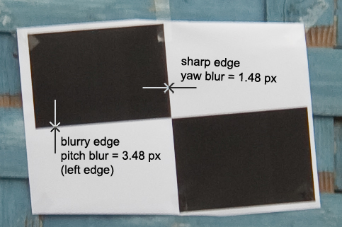
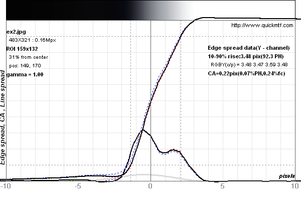
Fig. 2 A center crop from a photo taken with the slanted edge test method to measure shake blur (cf. wp „Understanding Image Sharpness“). Plus a plot of the LSF in pitch direction (Image #4158).
Tested camera: Pentax K-7 specimen #3, tester #3, Sigma 12-24 mm F4,5-5,6 EX DG lens at 12 mm, f/8.0, 1/80s, ISO 100, distance 150 f, 483x321 px2 large crop from original (aka 100% crop), type-C tripod, 0°, mirror lockup, remote trigger, no shake reduction, raw with „Sharp Setting“ (cf. wp).
The distance between the two peaks of the LSF is ˜ 10 µm (2 pixels).
2. Statistical collection of evidence
Our first examination to make sure that the shutter has a significant effect on image sharpness at all is to exclude all kinds of artifacts from our evaluation, like a defect camera, a „Parkinson'“ tester, a loose lens element, a bad day etc. The following testers (with cameras and lenses) have contributed to a solid data base:
-
Peter Smith (K-7 specimen #1, lenses: Pentax 50 mm)
-
Rüdiger Neumann (K-7 specimen #2, lenses: Pentax 16 mm, 31 mm, 135 mm, 300 mm rd)
-
Falk Lumo (K-7 specimen #3, lenses: Sigma 12 mm, Pentax 300 mm)
-
Henning Rink (K-7 specimen #4, lenses: Sigma 10 mm)
The data of Peter Smith have already been made public in a PDF document linked from the Pentax SLR forum at dpreview.com. We simply reuse his public data. All other data are unpublished.
We have studied the impact of the firmware version on the phenomenon. We compared, in particular, the following firmware versions:
-
1.02.00.16
-
1.03.00.22
and found no significant difference. Most of tests are done with the #22 release.
It is impossible to list all ~5000 measurement values (one to four measurements per photo) in this report. Therefore, we first do a condensation of all available results into a single chart of mean values of blur widths. To present the data with as little bias as possible, we present the total average blur widths prior to subtraction (Kodak p=2) of any static blur offset. The averages are taken over between 10 and 150 test shots each.
We differentiate between the blur width in pitch direction (which makes a horizontal edge blurry) and in yaw direction (which makes a vertical edge blurry). And we differentiate between disabling and enabling the shake reduction (SR). For the condensed chart, we take the average of pitch and yaw blur as follows:
b2 = ( b2pitch + b2yaw ) / 2
Note that this formula differs from the one to derive the blur angle. The following chart is obtained:
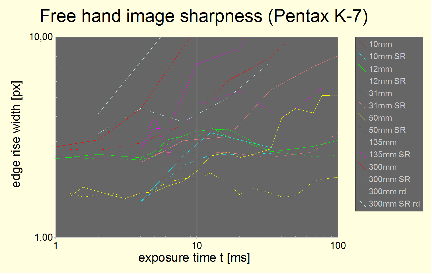
Fig. 3 Overview of average image blur, based on 4 testers, 4 K-7 cameras, 8 lenses and thousands of accurately measured test shots. The 16 mm data are missing from the chart but no different. Static blur offsets are not subtracted. The individual testing series lead to different static blur offsets varying between 1.5 and 2.5 px which is pretty normal and well explained. Blurs in excess of 10 px and exposure times in excess of 1/10s are not shown. Curves from the same lens use the same color, with SR values being dotted lines.
The statistical errors are smaller than average for 12 mm, 50 mm and 300 mm.
It may be worthwhile to note that for focal lengths of 31 mm and longer, the efficiency of shake reduction is quite obvious. For shorter focal lengths, it is efficient for sufficiently long exposure times.
Hint: For the html version of the paper, you may open an image in a separate tab and obtain better resolution (copy-paste the image URL if using Internet Explorer).
2. 1. Discussion of results from statistical analysis
It is clear from the above that there is extraneous image blur not explicable by regular free hand shake. Regular free hand shake should vanish with vanishing focal length and be a strictly monoton increasing function with both, exposure time t and focal length f.
However, in a region of about 5 ms = t = 33 ms (corresponding to 1/200 s = t = 1/30 s) there is a clear local „hill“ of extraneous image blur for focal lengths f = 16 mm for both, SR enabled and disabled. For f = 135 mm one has to consult the SR enabled curve to see it. Probably simply because the SR reduces free hand shake enough to not mask the smaller effect in the hill, whatever it may be. At f = 300 mm, the effect isn't statistically significant anymore and probably completely masked by free hand shake.
Nevertheless, the data for all focal lengths is compatible with the assumption that the total blur is basically the combination of three terms:
-
a static blur offset, constant in both f and t
-
a free hand shake blur term, approximately proportional to f*t
-
an extraneous blur term, constant in f but not t.
Looking at the data, we can conclude that the extraneous blur term has a maximum around 12 ms (1/80 s).
Finding #1: There is a statistically significant effect for shutter times of 1/80s ± 50% which on average leads to extraneous blur in images taken by any Pentax K-7.
Now that we verified to observe a common phenomenon present in all K-7 cameras, we can narrow our discussion to focal lengths less affected by free hand blur. Notably 10 mm, 12 mm and 16 mm.
3. Ultra wide angle analysis
3. 1. 10 mm
All results obtained with the same Sigma AF 10-20mm/F4.0-5.6 EX DC lens at 10 mm (465 g).
We now will analyze the blur width in pitch direction (blurry horizontal edge, abbreviated „-h“ in charts) and the blur width in yaw direction (blurry vertical edge, abbreviated „-v“ in charts) separately from each other. On average, this makes each of them smaller than the combined average which contained the static blur offset times sqrt(2).
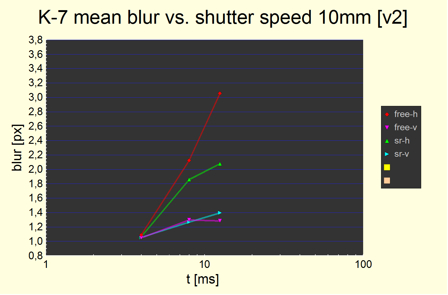
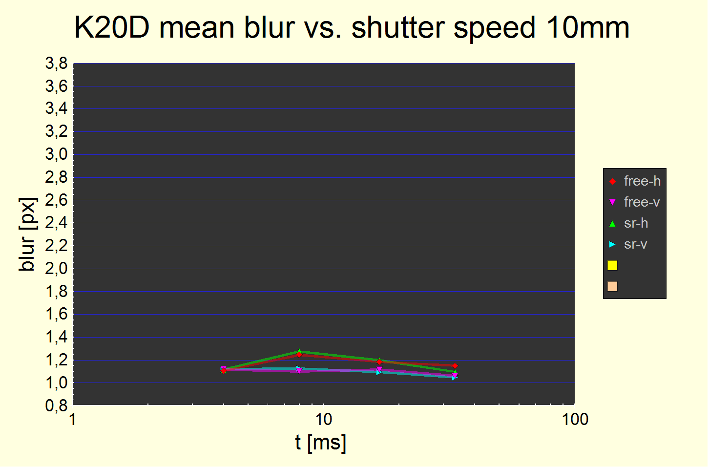
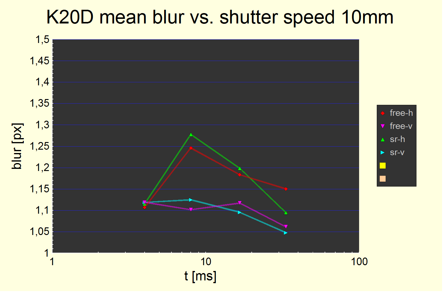
Fig. 4 Blur widths at 10 mm. Each chart has split curves for pitch (-h), yaw (-v), shake reduction disabled (free-) and enabled (sr-). Static blur offsets are not subtracted.
The first is for the K-7, the second and third for the Pentax K20D, with the second sharing the same scale as the K-7 plot and the third having a more appropriate one.
There is a clear peak in the K-7 pitch blur data at 1/80s (longer exposure of 1/60 s and 1/30 s not shown in this plot but it is smaller – look at the overall plot).
The effect is independent from shake reduction being enabled or disabled (the difference is not statistically significant) and affects almost only pitch blur, not yaw blur. The extra pitch blur at 1/80s is about 1-1.5 px (using the imprecise linear difference).
This is contrasted by the K20D data which shows a minimal effect which peaks at 1/125s and has an appearant amplitude of maybe 0.15 px, i.e., it is smaller than for the K-7.
The measured K20D pitch blur corresponds (Kodak formula with p=2) to 0.60 px or 3.0 µm. Which may be 4.3 µm at 1/180 s. Which is about 1/3 of the effect for the K-7 (cf. below).
We believe the cause for the minimal effect for the K20D to be the effect from the travelling mass of one or two shutter curtains. All SLR have this. Theoretically, it should peak at 1/180s. Our testing methodology is accurate enough to measure it.
Finding #2: The effect has no universal magnitude for all cameras. It is rather large for the K-7.
Finding #3: The effect causes blur in almost one direction only, the pitch direction (-h). A 2-norm averaging over pitch and yaw blur (as suggested by statistical models) will yield an underestimation of the effect. We don't do it in subsequent charts (but did in fig. ).
3. 2. 16 mm
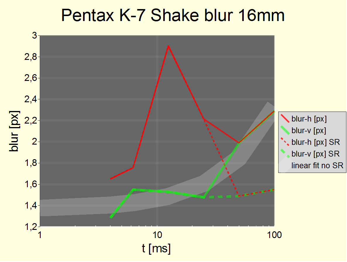
Fig. 5 Excess pitch blur at 16 mm. Mean values. SR disabled/enabled results are combined into one figure as their difference is not statistically significant at t = 25 ms. Static blur offsets are not subtracted.
At t = 50 ms (1/20 s), the free hand blur starts to become significant and SR has a significant and positive effect which masks the pitch/yaw blur difference. This is why both figures are then combined into one (the difference is still there but not statistically significant anymore – so not shown).
The tested lens is the Pentax DA* 16-50 F2.8 lens at 16 mm (565 g). The results at 16 mm confirm the 10 mm result. Its amplitude of 1.4 px confirms the 1-1.5 px measure at 10 mm. Note that this is from a different tester, different camera, different lens, different blur width measure software than at 10 mm. The only constant is the camera model: K-7.
Note that an average blur width of almost 3 px means that on the worse side of things you'll find blur widths of 2.9+1.4 or 4.3 px. Seeing the corresponding examples with your own eyes is a rather desillusioning experience. Remember the (less dramatic) example in the opening section?
3. 3. 12 mm
The tested lens is the Sigma 12-24mm F4,5-5,6 EX DG lens at 12 mm (600 g). By far the most precise measurement is available for 12 mm. Yet again another tester, camera specimen and lens. It is based on a thousand test shots or so. Below is a summary of results:
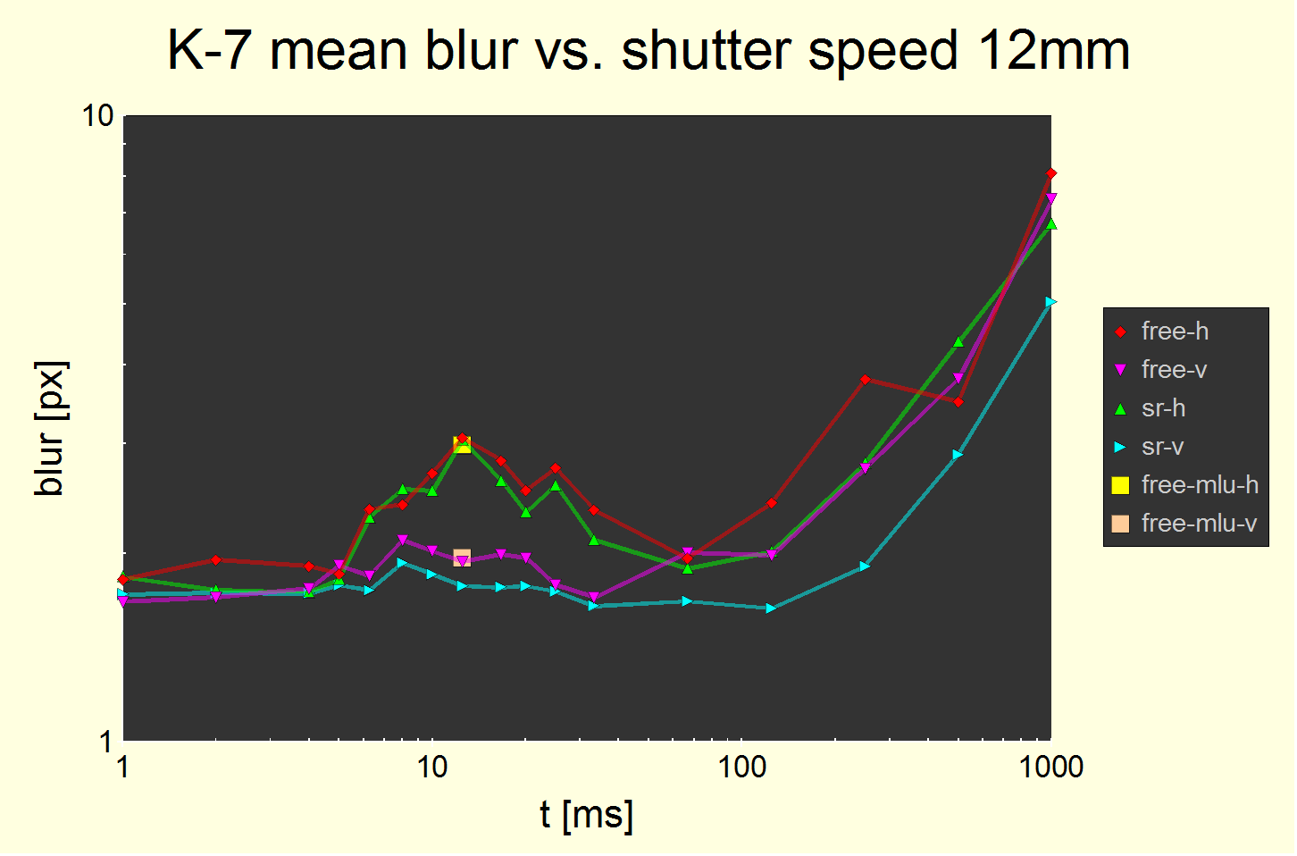
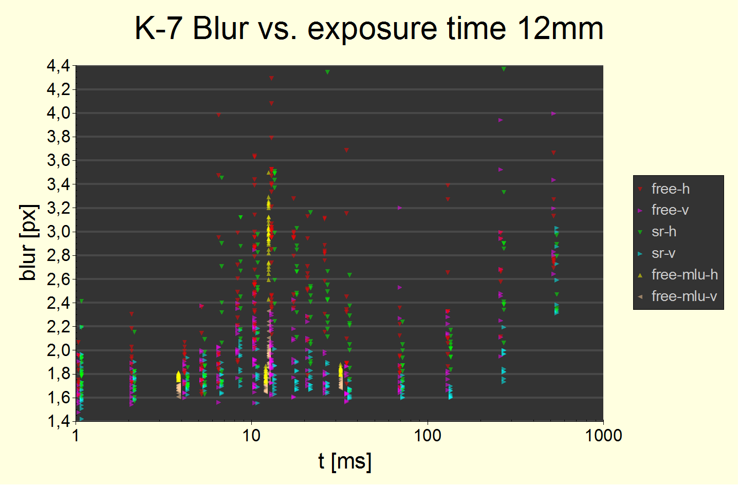
Fig. 6 Excess pitch blur at 12 mm. Mean values. Static blur offsets are not subtracted. At t = 33 ms, the difference between pitch and yaw blur dominates, at t = 67 ms, the difference between SR enabled and disabled.
At 12.5 ms, two additional precision measurements are shown: Free hand with 2 s timer which includes the mirror lockup feature (MLU) and disabled SR (square boxes). The impact of enabling MLU and disabling SR on extraneous blur is zero.
Fig. 7 All edge blur widths plotted, unaltered as they come out of the measurement. There are three additional MLU data point series (yellow and sand) which are to be ignored for the time being. The chart is clipping for large t > 100 ms. The difference between pitch and yaw blur is significant even at the level of the individual measurements, i.e., the „-h“ points (red and green triangles pointing down) are almost all above the „-v“ points (magenta and turquois triangles pointing right).
The variance is clearly visible as well: i.e., you'll always be able to find „good“ counter examples where pitch blur is untypically small like only 2.0 px which is close to the static blur offset of 1.7 px. However, this is a statistical effect unfortunately not negating the effect. On the opposite end, there are really bad examples exceeding 4 px blur.
The results at 12 mm confirm the 10 mm and 16 mm results. Its amplitude of 1.3 px again confirms the 1-1.5 px measures. We will later see however, that the real amplitude of the effect is larger as it is masked partly by static blur (2.2 px to be precise, to be discussed later).
Finding #4: If not masked by free hand blur, then the effect is almost independent of focal length.
4. Testing for alternative causes
4. 1. Mirror slap or shutter release button finger movement
Finding #5: The effect is not caused by mirror slap or shutter release button finger movement.
This much we could already find out from the analysis as carried out so far, esp. fig. . Eliminating both factors has zero impact on the results. Now, we will narrow down the search for possible causes.
4. 2. Vibration
Parts in the body (or lens) could vibrate, e.g., due to operation of the focal plane shutter. Let's call this the „bell effect“.
A later high precision accelaration measurement will reveal the K-7 frame (the „bell“) resonance frequency to be about 900-1000 Hz. You can actually hear it if you hit the tripod screw hole and listen with your ear nearby.
In order to check for or against it, we mounted the camera to a class A tripod (cf. white paper classification of tripods). The results are shown below:
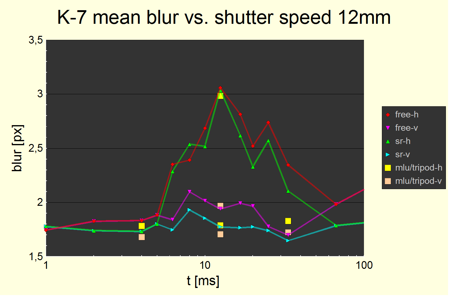
Fig. 8 Same as fig. but with 2 additional mean blur data points at each of t=4 ms, 12.5 ms and 33 ms, taken with a class A tripod. Static blur offsets not subtracted.
We may ignore for a minimal systematic 0.11 px difference between „-h“ and „-v“ measurements which are probably due a slight decentering artifact in the lens. After all, it's „only“ a Sigma ;) It would be easy to correct for the effect but leave it alone as it really isn't worth it.
Having said this we see that a class A tripod entirely eliminates the effect.
Finding #6: The extraneous blur is not caused by a bell vibration effect. It is caused as a result of extraneous body movement during the exposure.
Note: this finding does not rule out a vibrating imaging board (which the SR module is mounted onto) where vibration is stimulated by body movement rather than frame vibration. Therefore, whenever we consider vibration of the image sensor in the following, it could be caused by mechanical vibration of the imaging board too. But it does rule out an effect such as air flow interaction between image sensor and shutter curtain or mirror.
4. 3. Shutter curtain travelling mass
So far, we found that the extraneous blur is caused by movement of the camera body. The mass and velocity of the travelling curtain segments can be some hundred mg and cause a counter movement of the body as mandated by the conservation of linear and rotational momentum. With a vertical blade shutter, the pitch direction of movement would match. Let
? (t,t) = min (t/t, t/t)
be an excitation function which has its maximum of 1 at t=t. Then, we should roughly obtain:
bshake (t) = a ? (t=1/180 s, t)
because the maximum effect is obtained if the shutter keeps moving for the entire duration of the exposure. Which is the case at the flash synchronisation time (or slightly less). The data for the K20D would be compatible with such a behaviour (cf. fig. on p. ). But let's say that the available data cast some doubt on this cause for the K-7. Let's look at only the pitch blur data, SR enabled and disabled combined to improve accuracy even further (the SR setting was shown to have no significant effect):
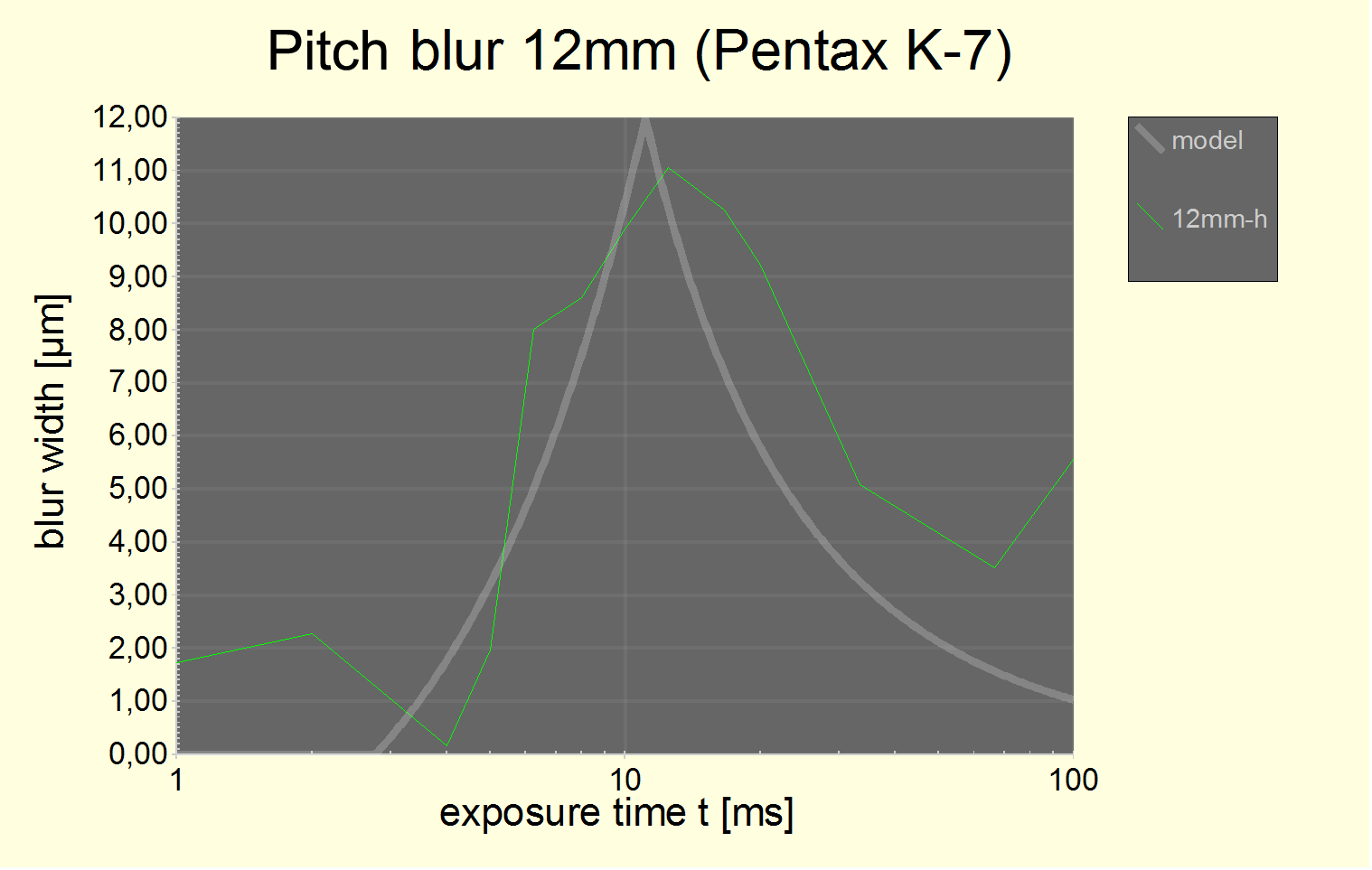
Fig. 9 pitch blur with static blur offset subtracted using the Kodak formula with p=2 and expressed in µm for 5µm large pixels. At t = 1/13 s we see the then non-zero effect from hand shake at f=12 mm. The absolute error in the data is larger for small values.
The fitted
model curve is bshake(t) = a ? (t-t0,
t-t0)
with
a = 12 µm
t =
1/90 s
t0
= 1/360 s
The travelling shutter formula (t0=0 and t=1/180 s) would just not fit. Even using a shifted curve with the parameters above, the fit is bad.
Note that we measure blur at the image center. t0 = 1/360 s corresponds almost exactly to the time where the image center is still exposed when the first shutter curtain stops. From the curve above, it could be that the extraneous blur builds up between t0 and 2 t0 (a time span of 2.8 ms) and the visible effect is maximized at 4 t0 when the old and new images (pre-t0 and post-2 t0) superimpose with about same magnitude.
Finding #7: The extraneous blur may or may not be caused entirely by the momentum of moving shutter curtain blades. More likely not.
But we are sure that the shutter plays a rôle in all this. At the moment in consideration (t0 = t < 2 t0) no other movement takes place. That's the reason for the title of this paper too.
4. 4. Extraneous blur parameterization function
If the extraneous blur is not caused by travelling masses then the travelling shutter function ? (t,t) is a bad parameterization. The data are actually better described by
? (t,t) = 4 t t / (t + t)2
which like ? (t,t) has its maximum value of 1 at t=t and starts linearly at t=0 and falls off proportionally to 1/t for large t.
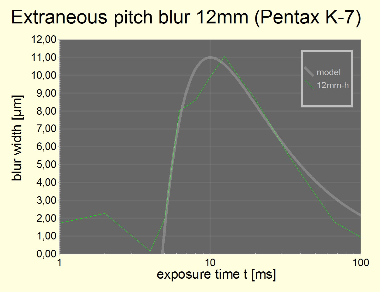
Fig 10 Extraneous pitch blur with static blur offset and free hand blur subtracted using the Kodak formula with p=2 and expressed in µm for 5µm large pixels. The absolute error in the data is larger for small values. In order to subtract free hand shake, we only used SR data for t = 16 ms and used the 3 mrad/s shake reduced angular velocity parameter.
The parameterized model
curve is bshake(t) = a ? (t-t0,
t-t0)
with
a = 11 µm
t =
1/100 s
t0
= 4.8 ms
Within data error margins, the model seems to be about 90% correct.
The above parameterization is useful to predict camera performance.
4. 5. Estimation of body acceleration
An assumption of shutter curtain travelling mass directly causing the extraneous blur effect leads to a bad fit of data but wasn't excluded.
A short calculation reveals that inertial masses involved to cause any effect in excess of 0.5 px or 3 µm (such as found for the K20D) require a shutter with an effective mass of travelling parts in excess of 300 mg per curtain. To explain the effect as seen with the K-7, an effective mass of 1 g would be required, corresponding to an overall shutter weight of 3-5 g. An APS-C focal plane shutter shouldn't be this heavy but one never knows...
4. 5. 1. Body mass dependency
We did a comparison test with a DA*16-50 vs. an FA 17-28 (600 g vs. 255g; or 1350 g vs. 1000 g incl. body weight).
The results (linear difference between pitch and yaw blur) are:
1350 g: 1.06 px
± 0.08 px (error of mean value)
1000 g: 1.34 px ±
0.10 px
This difference is compatible with an assumption that the extraneous blur effect is inversely proportional to body weight which means proportional to shutter weight.
4. 5. 2. Smoothed body acceleration
In order to estimate the effect of travelling shutter masses, one of us decided to measure the body acceleration (cf. fig. ). The resulting accelerations have a strong harmonic component (of about 1 kHz frequency). Therefore, we first present the results where accelaration is filtered with a Gaussian square kernel with 1.2 ms standard deviation (2.4 ms width) (cf. fig. ).
The smoothed body acceleration data are on the heavy side of things. If the shutter would move at constant speed, then 5 mm/s correspond to an effective shutter curtain mass of 1500 mg; if it is smoothly accelerated and decelerated, then it would be 700 mg. An effective shutter curtain mass of 1000 mg could be heavy enough indeed to explain the magnitude of the K-7 extraneous blur effect.
However, we did the same test for the K10D and it performs very similiar, maybe 2/3 of acceleration and velocity values.
An exact look into the curtain acceleration curve is interesting though: Increasing acceleration from 0-3.7 ms (3.7 ms), decreasing acceleration from 3.7-5 ms (1.3 ms) and deceleration from 5-6.5 ms (1.5 ms) followed by a hard stop and about 2 ms settling time. This looks like motor-driven shutter deceleration and a hard end stop which must absorb a fraction of the shutter blades' motion energy only. This does mean too that the shutter velocity is maximal in the middle of the travel rather than the end.
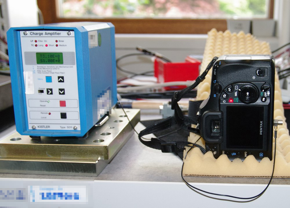
Fig. 11 One of several body acceleration measurement setups. The acceleration sensor is glued onto the tripod mounting hole.
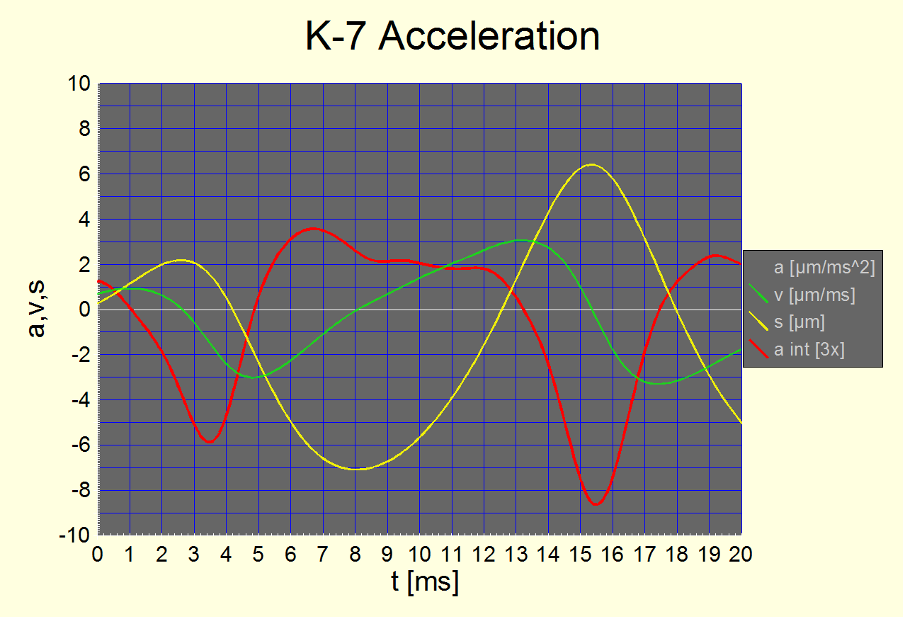
Fig. 12 Body acceleration (K-7) where t=0 corresponds to the start of the first shutter curtain.
Velocity v and position s are integrated from acceleration a. Acceleration settles at about 2/3 m/s2 (which should be read as 0) between 8 and 12 ms which is about the time between stop of first and start of second curtain. The local maximum at 6.5 ms is the audible shutter click's main component.
It almost looks like the shutter blades are decelerated after 3.7 ms when acceleration is maximal. At that time, the shutter blades are in full motion and in the middle of their travel. Here, the maximum difference in body velocity is 4 mm/s. The measurement is not perfectly clean as external sources of acceleration are seen to exist.
A single frame from a 1000 fps hi-speed camera (cf. section „Shutter detail„ on p. 25) reveals that a shutter blade in the middle of the action moves 7 mm within 1 ms (1 frame)! Relating this to 5 mm/s max. body velocity yields an effective shutter curtain mass of ˜ 700 mg and a body displacement of ˜ 10 µm.
Finding 8: The effective travelling shutter mass per curtain is about 700 mg. The (irrelavant) total shutter mass may then be about 3 g. The figure isn't very accurate (500-900 mg) but good enough.
Note that body displacement and blur width are different due to a rotational component around the body+lens combination's center of gravity.
4. 5. 3. Full body
acceleration
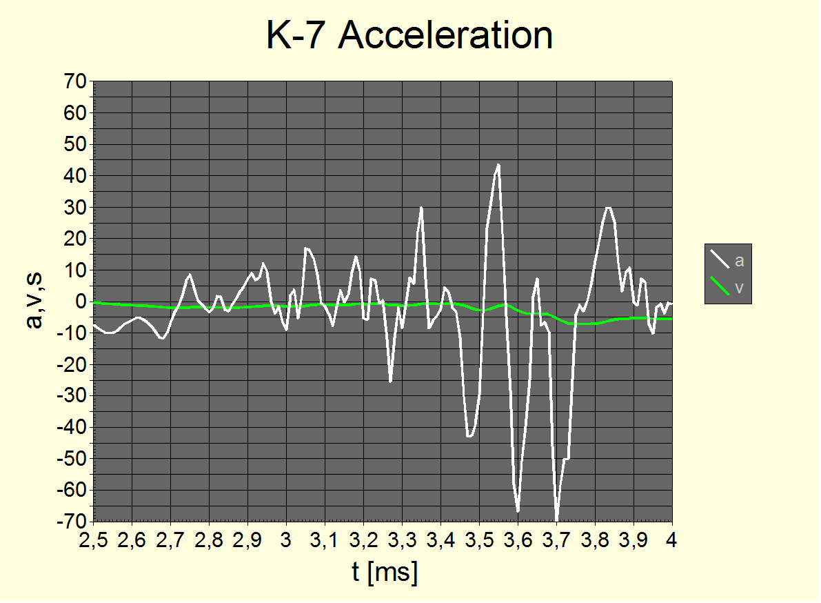
Fig. 12 The above chart shows the full acceleration values sampled at 100 kHz and filtered at 30 kHz. This is the moment of maximum 7 G body acceleration (3.7 ms after start of curtain 1).
It is clear that the body forces which the shutter creates are high, up to 7 G!. The majority of these forces are absorbed by body vibrations though which seems to have a resonance frequency of about 1 kHz (which is audible if you listen carefully!). Averaging over 0.1 ms, the maximum acceleration still is 3 G. It is safe to assume that inner body parts see accelerations in excess of 1 G over 0.1 ms or longer.
A comparison with the K10D reveals no striking differences, which we measure accelerations in excess of 5 G for.
Finding #9: The K-7 shutter may be heavy and fast enough to explain a good part of the extraneous blur effect, maybe a 1.5x increase compared to the K20D which then would amout to about 50% of the total effect. But it isn't heavy and fast enough to explain all of the effect. There must be another factor to explain it. This is the author's collective assessment.
Note: To accelerate 700 mg to 7 m/s within 3.7 ms with linearly increasing acceleration results in a final body acceleration of 0.27 G, as about shown by the smoothed acceleration curve.
4. 6. Second order shutter effects
We will try to determine what shutter effect exactly causes the extraneous blur. First, we designed a decision experiment:
If the camera is reversed upside down (180° landscape orientation) then the expected first order effect (from the travelling masses) shouldn't change at all. If we see an effect then we got new information input for our analysis. We have run this experiment using a class C tripod. It has the advantage that it further reduces measurement variations and allows for automated testing routines. The first finding is that in 0° landscape orientation, a class C tripod exactly reproduces the free-hand extraneous blur effect. This was to be expected because we deal with extremely small and fast body movements:
The experiment's outcome speaks a clear language: The extraneous blur effect at 1/80s is increased by turning the camera upside down. The amount of increase varies on the kind of edge being evaluated: It is between 0.3 px and 0.6 px stronger, which is a 30% to 60% effect and statistically highly significant.
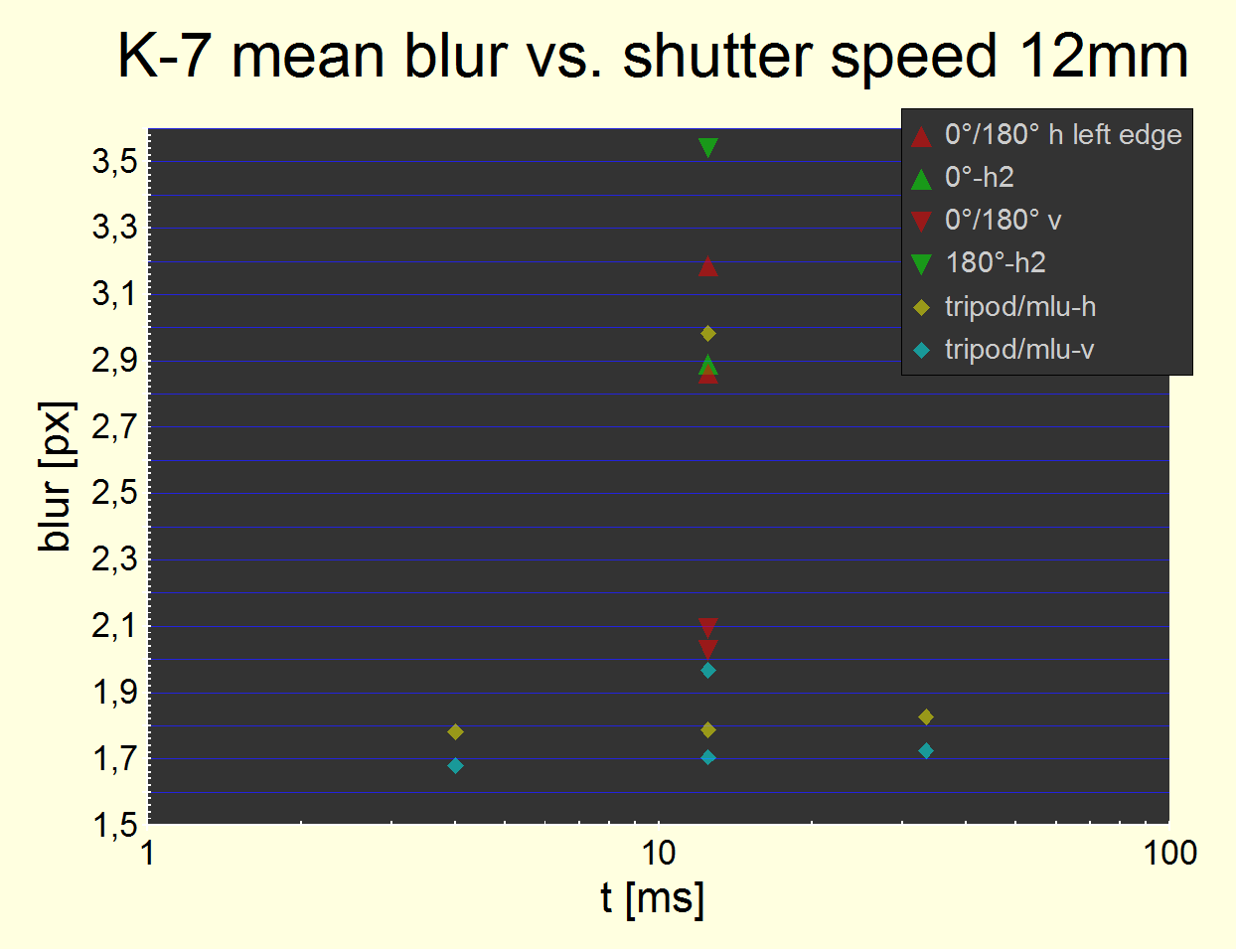
Fig. 13 An independent measurement at t=12.5 ms using a class C tripod (red and green triangles) and comparing with already presented results for the class A tripod (lowest six data points) and free hand with 2 s timer and MLU (the upper sand and turquois diamonds, 12.5 ms only). Static blur offsets not subtracted.
The chart is a bit awkward to read: In the 12.5 ms column, from top (worst) to down (best), we have:
1. Upside down
pitch measurement of the right horizontal edge (180°-h2).
2. Upside down pitch measurement of the left horizontal edge
(180°).
3. The previously existing 2 s-timer/MLU normal 0° pitch
measurement (sand diamond) at about 3 px.
4. Normal pitch measurement of the right horizontal edge
(0°-h2).
5. Normal pitch measurement of the left horizontal edge (0°); #3,
#4 and #5 are almost the same.
6. Upside down yaw measurement (180°).
7. Normal yaw measurement (0°).
8. The previously existing 2 s-timer/MLU normal 0° yaw
measurement (turquois diamond).
9./10. Normal 0° pitch and yaw measurements with a class A
tripod.
The following figure shows all individual measurements for the 180°-h2 and 0°-h data:
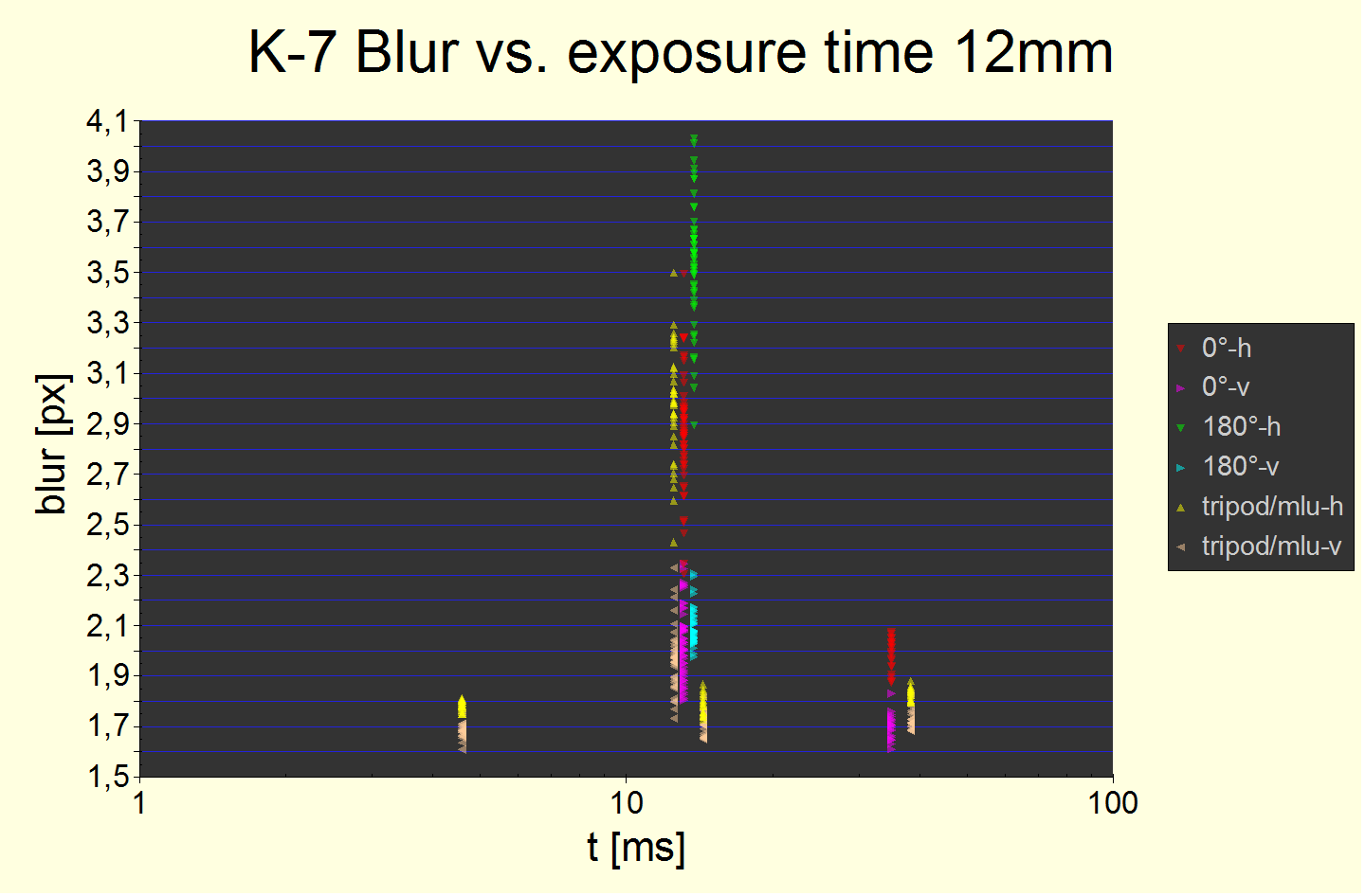
Fig. 14 Raw measurement data. The increase of the effect by turning the camera upside down is very visible (green down triangles for right horizontal edge 180°-h2). Static blur offsets not subtracted. It is certainly statistically very significant.
Let's now understand the dependency on the kind of edge. Normally, the blur width should be the same independently of whether we measure the left (white-to-black) or right (black-to-white) horizontal edge. However, the application of the „Sharp Setting“ introduces non linearity into the process. The measured width will depend upon whether the blurry slope or double line is more into the black or into the white. So, the blurring effect isn't constant over the exposure time. We get different measures for both edges if the effect is not centered around the middle of the exposure time window. The following is a correlation plot of left vs. right edge blur widths:
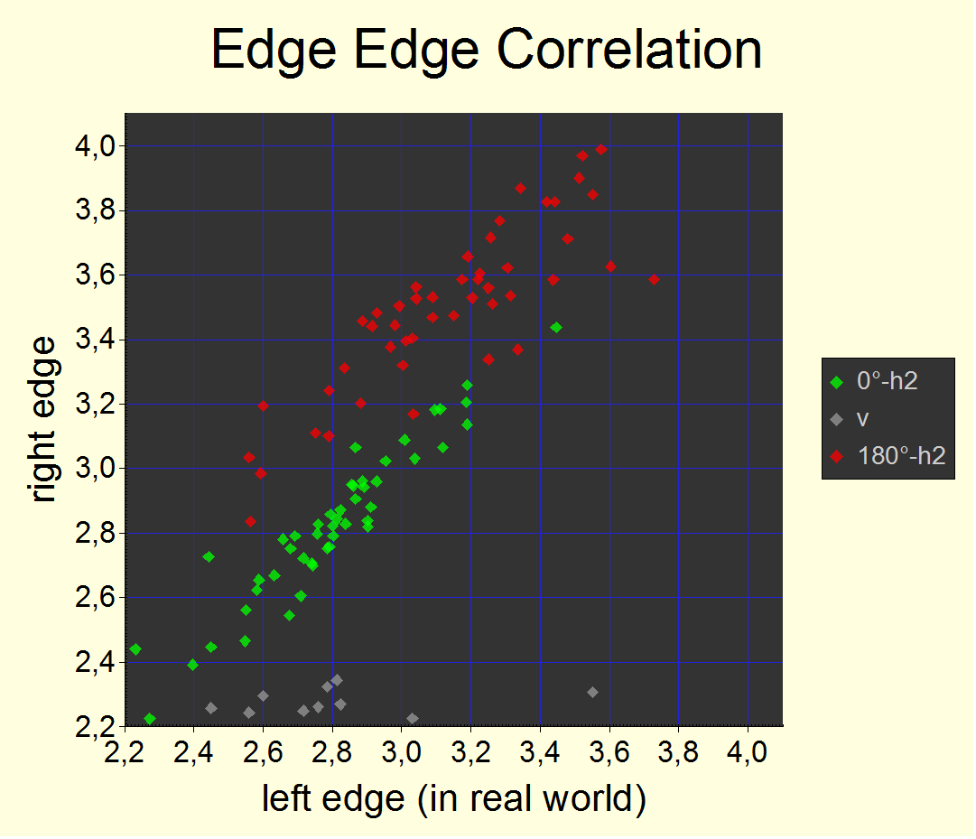
Fig. 15 Left vs. right horizontal edge pitch blur correlation at t=12.5 ms. As one can see, for normal 0° landscape orientation, we get no significant difference which is an indication that the effect happens towards the middle of the exposure time interval. The difference between red and green is obvious.
For 180° upside-down orientation, one edge is measured to be more blurry than the other (and both are larger as well). From that we conclude that the effect happens time-shifted with respect to the middle. So, for upside-down operation, we're probably not even hitting the maximum at t=12.5 ms. It is difficult to reason though if it happens earlier or later than at 0°.
The edge-edge correlation was an important analysis to rule out that the increase of blur width when rotating the camera upside down is simply an effect of measuring the „other edge“. It is not. The effect is real and not explainable by systematic measurement errors.
Overall, we conclude that reversing the camera increases the extraneous pitch blur at 12.5 ms by about 50%.
Finding #10: The extraneous pitch blur is caused by body movement which is not entirely due to travelling curtain counter movement. Because otherwise, it would obviously have to be independent of orientation.
But the shutter is the only moveable part to be at the beginning of events.
So, we think we have other candidates for the cause now: It may be related to a part in the shutter hitting hard when the curtains stop. This happens after 1/180 s, i.e., 1/360 s after begin of exposure of the center. And causes an effect we have to further investigate now.
Independently or additionally, it can be related to an interaction during the phase of fastest curtain movement and highest body acceleration.
5. The shutter interactions
5. 1. Shutter stop
We named the shutter stop as a possible root cause. However, it cannot be as simple.
When the shutter stops, all remaining travelling masses (which have been accelerated and decelerated moderately to up to 7 m/s and down to closer to 0 m/s again) are stopped with high deceleration. But this wouldn't be a problem. Because the combined effect on body movement cannot be larger than that of acceleration. And this was already shown to be insufficient to explain the effect on its own and independent on orientaion. We talk about 700 mg which find an immediate halt.
Below is an acoustic analysis of the process:
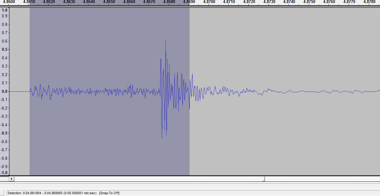
Fig. 16 The noise of the moving shutter, first curtain. After 6.55 ms (1/150 s) there are signs of an impact. It makes the K-7 shutter almost as loud as the (dampened) mirror slap noise. We take this as a sign that the shutter movements are eventually stopped hard (it happens at precisely that moment).
BTW, the shutter opens exactly 18.6 ms after the begin of mirror flip operation.
Finding #11 The aperture lever motor, lens aperture or electromagnetic sensor fixation drive cannot contribute to the effect. The aperture is closed in parallel with the mirror flip operation or MLU operation. There really are no other moving parts involved we could make responsible (w/o SR). At that moment in time, there are no parts draining excess electrical power neither.
So, if it isn't the effect of conservation of momentum then it must be a direct consequence of deceleration. The deceleration may be high but extremely short.
A short calculus shows that deceleration can be as high as several thousand G when the shutter stops hard! (It already is up to ~400 G during normal acceleration...) But only for a very short period of time like 0.1 ms. Which is why it isn't normally a problem. However, it makes the body accelerate for the same amount of time, with an acceleration which is reduced by the ratio of masses (which may be about 1250 g/700 mg or 2000). So, this leaves the body with an acceleration of a few G for a fraction of a ms. Even at 3 G, the body does only move by 0.15 µm which is only 1% of the effect we observe. Acceleration forces exceeding thousand G are quite common in precision engineered machine parts. Steel and the all metal framing of the K-7 body are stiff enough to create and propagate high G forces through the body. And now, it's clear too why a class A tripod (clamping to a stone table) helps: it prevents the body from acceleration as the stone table has a huge mass.
5. 2. Shutter curtain acceleration
The acceleration measurement has shown that the stop isn't the only high acceleration phase during shutter operation. Another phase is at 3.4-4 ms when the shutter curtain reaches its highest velocity and switches from increasing to decreasing acceleration. The curtain acceleration then „only“ is about 400 G and body acceleration is about 0.3 G rather than 3 G. But it is maintained for 1 ms rather than 0.1 ms and its overall effect may be just as large. Moreover, the extreme short term 0.01 ms spikes of highest 30-70 G body force happen during this phase.
We summarize this by saying that the body is encountering a momentum of 0.3 G x ms or 3 µm/ms.
So, the question is: What part in the Pentax K-7 may get into trouble if body momentum exceeds a threshold? And now all of a sudden it is clear: the maximum magnetic driving G-force for the sensor may be exceeded.
Finding #12: The shutter operation creates body acceleration forces which do temporarily (between about 0.1 ms and about 1 ms depending on camera orientation) exceed the maximum magnetic force of the image sensor driver.
Below, we will study the consequences of this finding in more detail. First however, let's take a break, look at the shutter and let's understand where the high acceleration forces are coming from.
5. 3. Shutter detail
Direct link to 1000 fps hispeed movie: MP4 (2 MB)
Before we proceed, we must verify that all our deductions hold true.
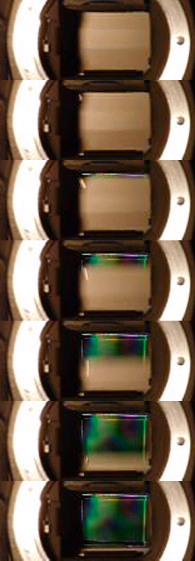
The image sequence to the right is from a high speed film sequence of the opening shutter. The frames are 1 ms apart. So, the sequence is about 6 ms long and the loud shutter noise indeed is from the impact at the end.
The curtain travels top to down. Well, this was predicted as written in section 5.4 on p. 27 and in our work, the prediction was first ;)
In the opening and closure sequence, we can see parts of the levers which hold the three blades in place. Here, we see the back part of a micro bolt and not the actual lever. For the closing shutter, we can see the actual levers (and there are two of them for each curtain).
The follwing are superimposed images from the opening:
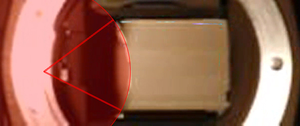 and closure sequence:
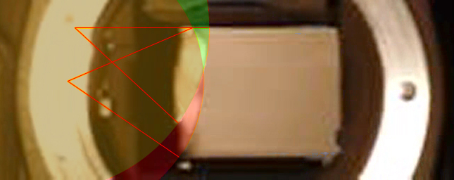 One can see that the levers
rotate around an axis, are about 20 mm long and that there are
four of them. We can compare this to other known shutter designs,
e.g. a well known focal plane shutter with 3 down-travelling
curtain blades:
One can see that the levers
rotate around an axis, are about 20 mm long and that there are
four of them. We can compare this to other known shutter designs,
e.g. a well known focal plane shutter with 3 down-travelling
curtain blades: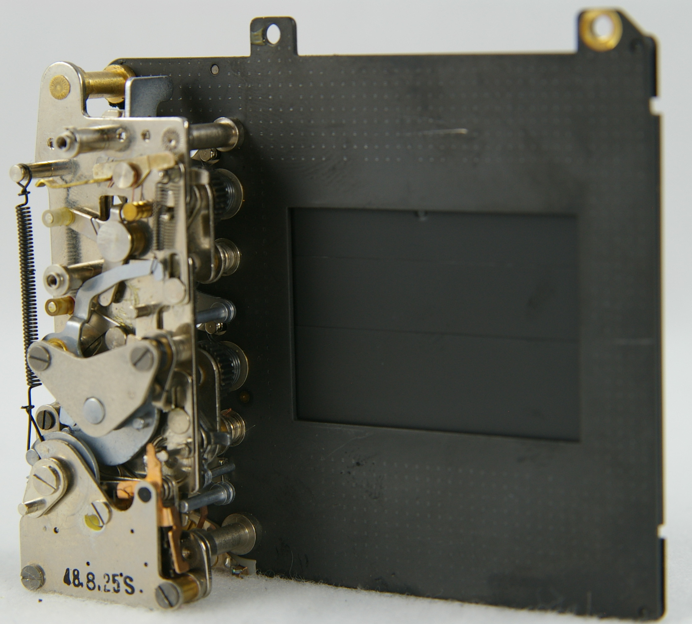
Fig. 17 Focal plane shutter with four lever axes (visible at the right side of the left metal shutter mechanics, down near the curtain blades.
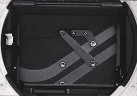
Fig. 18 Copal Square ES shutter with two levers per curtain and at least 2 microbolts per blade. When the shutter stops, both metal levers run parallel to the bottom edge and hit into the bottom metal cage.
Finding #13: The shutter is of the generic design with two full metal levers per curtain which may hit hard the bottom of the shutter when it stops. The levers are massive enough (a few 100 mg) to cause a shutter stop effect.
Also, the shutter is different from K20D's as this is required for its better performance. In the K-7, the levers are accelerated and decelerated by a driver. The levers don't hit the bottom at maximum speed. But they don't land soft neither. They are still rather „loud“ when they encounter their end of motion, only a few dB less loud than the mirror slap, actually ...
(Note: 2 steel levers of about 20 mm x 3 mm x 0.3 mm weight almost 300 mg!)
5. 4. The electromagnetic fixture of the „floating“ sensor
The image sensor is hold into place by electromagnetic force (an electromagnetic linear motor).
From the increased effect at upside-down, we can independently deduce that the shutter must hit from top to bottom, making the body accelerate towards the bottom and bringing Earth's gravity in a direction where to assist the electromagnetic force: The required force to hold steady the sensor is actually reduced by -1 G. Upside down however, the required force increases by +1 G, a difference between the two of 2 G. A difference which must account for an increase of the effect of at least 50%. So, we know that a few G are the right order of magnitude.
But, shouldn't the electromagnetic sensor fixture be much stronger anyway? We can give a lower bound for its strength:
We know that the SR mechanism supports 800 mm focal length lenses which at 10 mrad/s angular velocity (and a factor 2 for bad instances) require the sensor to move at 16 mm/s (although only for a short period of time). It must accelerate the sensor to this velocity within the 18 ms before the exposure starts. This is 0.9 m/s2 or 0.1 G. Adding normal G force and some safety margin and then there is no reason to believe the electromagnetic sensor fixture is stronger than maybe 1.5 G. So, e.g. 3 G down acceleration would leave 2 G for the sensor fixture to hold and would probably overload its capacity by 0.5 G. And 2.5 G in the other direction.
If it fails and the sensor „slips“, then we may see blur. However, still only in that magnitude of 3 µm as explained above. We still need to investigate this further.
Finding #14: The shutter curtains move from camera top to bottom (the direction of gravitational force for normal camera orientation). This initially was a prediction and needed verification.
Finding #15: A partly failure of the „floating“ sensor fixture is by far the most likely triggered cause (the root cause being the high shutter-deceleration induced body acceleration). However, it is not the final cause as its effect alone would be too small to explain what we see.
5. 5. The sensor positioning control loop
According to Pentax patent US20080226276, the SR device uses the Hall effect to register the image sensor location and to drive the linear motor such as to keep its position fixed (with SR off).
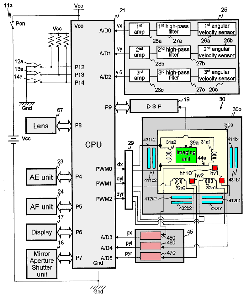
Fig. 19 Sensor positioning control loop according to patent US20080226276.
The three red squares are the hall sensors, the rose boxes are integrated circuits which send positional data to the CPU. The CPU computes and sends electromagnetic driving forces to the driver coils (turquois elements). The CPU is a Fujitsu Milbaut M-5 processor running at 132 Mhz or more.
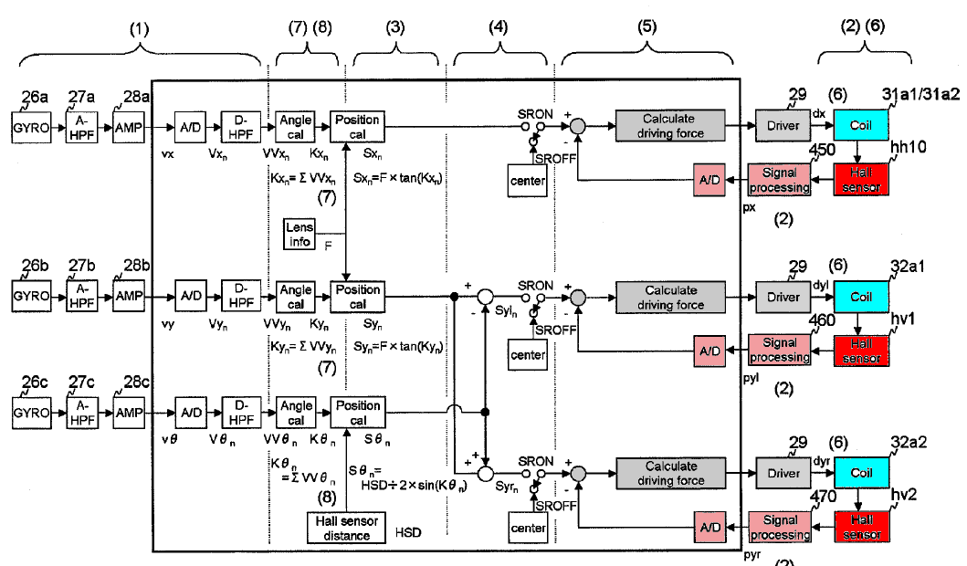
Fig. 20 Control loop for each coordinate direction according to patent US20080226276.
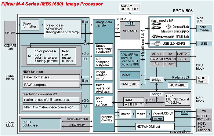
Fig. 21 Fujitsu Milbaut M-4 132 Mhz processor.
The Pentax K-7 firmware
image symbols as published on the internet contain no entry point
symbols to compute electromagnetic driving forces. It does however
contain symbols SRIC IN/OUT. Therefore, chances are that the
controller code is hardwired and not
running on the CPU
(e.g., Shake
Reduction
Integrated
Circuit).
We already found that the shutter has parts massive and is fast enough to accelerate the body by more than the floating sensor fixation force, e.g. when the shutter is in full acceleration or when it hits its stop. But why does the sensor move by such a large distance?
In order to evaluate it, we ran a simulation of the system camera + lens + shutter + hall sensors + electromagnetic driver + control logic + gravity.
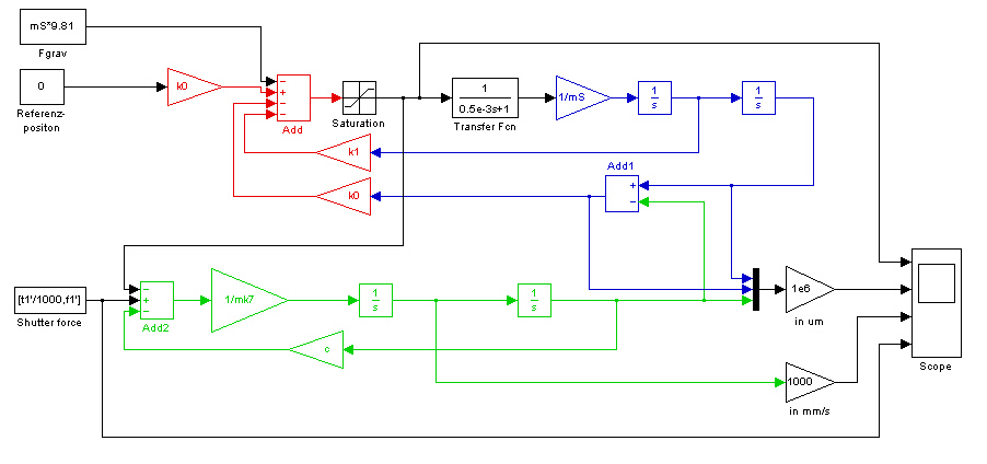
Fig. 22 Simulated control loop block diagram.
Our simulation uses a PD controller (proportional and differential) with the proportional correction force being:
forcecorrection (t) /m = -cx (x (t-?t) -x0 ) – cv (v (t-?t) -v0 ) saturated by ±Fmax
where x0 is such that the sensor is centered and v0=0. ?t is the combined controller and hardware response time and cx and cv are control variables. Fmax is the strength of the electromagnetic driver.
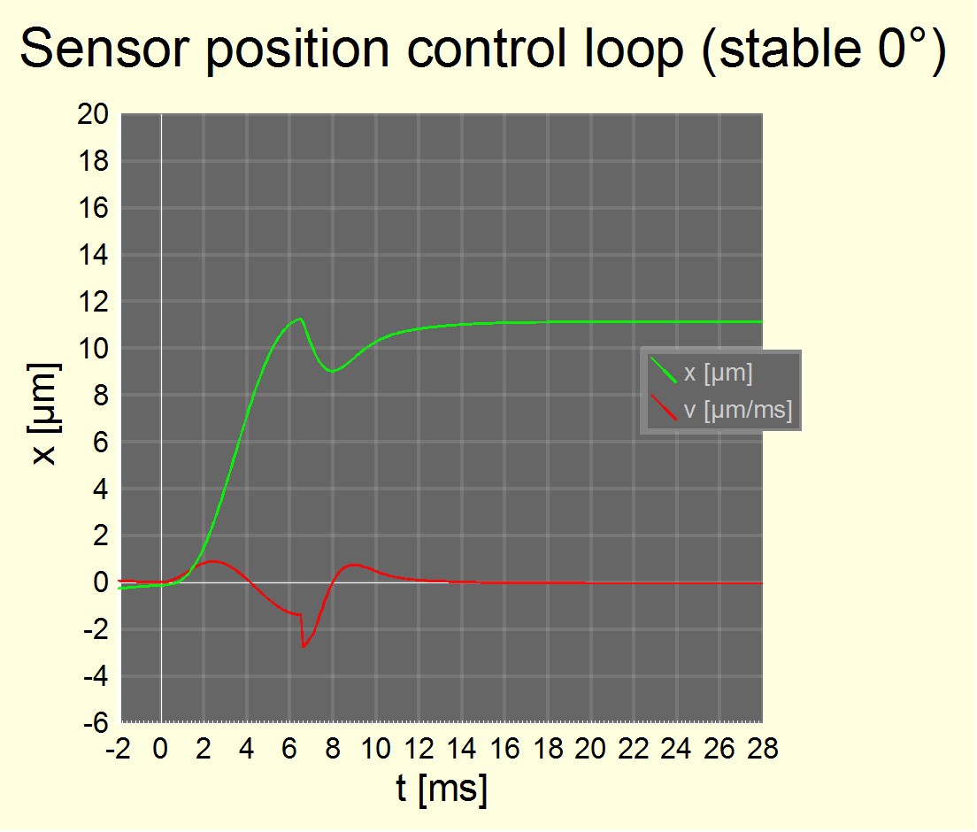
Fig. 23 Sensor positioning control loop simulation result with t=0 being the start of shutter curtain 1 travel. The controller parameters are as follows:
?t =
0.5 ms
Fmax
= 15 m/s2
cx
= 300,000 /s2
cv
= 1,000 /s
In the simulation, we assumed a shutter opening a 20mm window and with an acceleration which is harmonic with a period of 8.8 ms and a hard stop after 6.6 ms (¾ of its period, just when the shutter runs free). So, deceleration force is 50% soft and 50% hard. The effective curtain 1 travelling shutter weight is 700 mg and curtain 2 is left open (bulb mode). Body weight is 1250 g. No rotation about the center of gravity was assumed which isn't realistic. The green line is the absolute sensor position in the physical space, the red line is the sensor velocity with respect to the hall sensors.
The image sensor follows the body movement with a tad more than 1 ms latency and the overall system behaves like one with a fixed sensor. The body movement of 11 µm is due to the relatively heavy 700 mg effective shutter curtain, as seen with simple math: 0.7 g/1250 g*20 mm = 11 µm.
We know (from K20D/K10D blur/acceleration measurements) that image blur would be about half this value, probably due to a rotational component of body movement. In a chart like the one above, visible image blur should be maximal at 6.6 ms or 1/150 s.
The parameters in the chart above have been chosen to provide quick and stable convergence, e.g., to feature the ability to accurately move the sensor by large distances during its initialization phase. With above parameters, the sensor settles (± 0.1 µm) after travels of its center of gravity of 1 mm (40 ms) or 0.1 mm (18 ms). BTW, this is why the simulation doesn't start at zero excatly. It starts at -18 ms at begin of initialization. Parameters for Fmax and ?t are assumed system limitations.
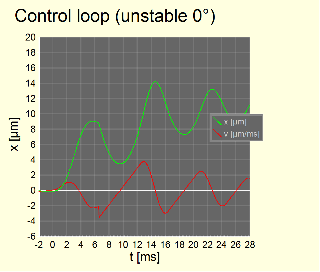
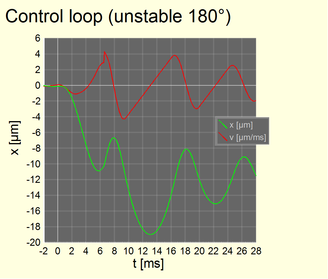
Fig. 24 Sensor positioning „sloppy“ control loop simulation result with t=0 being the start of shutter curtain 1 travel. The parameters are for a sloppier controller and deviate by about 50% from the parameters before, e.g., Fmax = 11 m/s2 and ?t = 0.7 ms.
The right chart is for 180° upside-down camera orientation and leads to 35% larger maximum sensor movement. The final sensor position still is 11 µm (must be) but it takes some 30 ms to reach it.
We have simulated a „sloppy“ control loop too, where parameters are close but allow for much slowlier convergence. It has the positive effect that the body movement due to shutter movement isn't fully transmitted to the image sensor and blur for exposure times less than about 1/100 s is reduced. But for larger exposure times less than about 1/60 s, it is increased, actually.
Most interestingly though, reversing the camera upside down now clearly can lead to more blur.
To be fair, we should note that the sloppy control loop is at the edge of an unstable controller and not likely to have been a design goal at Pentax. However, we cannot exclude that the real controller has similiar properties, maybe inadvertedly, and we conclude:
Finding #16: A „sloppy“ controller can lead to 30 % - 200 % more blur in images, keeping the sensor swinging between two positions for a couple of ms.
Note that the „sloppy“ controller case and the case of a mechanically swinging imaging sensor board (cf. above) are very similiar and cannot be distinguished.
Another possibilty are non-linear terms in the sensor positioning control loop. They can lead to arbitrary amounts of additional sensor movements and image blur. We cannot give limits in this situation except that it would strongly depend on the shooting situation.
An extreme case for a non-linear term is a software bug. Less extreme cases are common in PID controllers and square and higher order terms in non-proportional controllers.
Finding #17: The feed-back loop which tries to move the image sensor may or may not contain an ill-behaving non-linear term. If it does, it could explain the effect as well.
Such an ill-behaving non-linear term could be called „loss of traction“ which may be triggered by high velocity values which last for 0.1 ms or 1 ms only. However, if the control loop then behaves ill it may stay out of traction for an extended period of time and blur data strongly suggest this resettle time to be a few ms (remember t0?) rather than 0.1 ms.
We have one more result, from the images we started the article with: The edge blur's LSF (sometimes) shows two lines, i.e., two distinct sensor positions (10 µm apart) where the sensor stayed during about 50% of the exposure time (i.e., for about 6 ms each). This is incompatible with the stable and tight control loop's sensor positions over time. But compatible with the sloppy controller's positions. And most likely would be compatible with an ill-behaving non-linear term too.
5. 6. Shutter interactions summarized
-
The K-7 has a heavier and/or faster shutter than the K20D, creating about 50 % larger body accelerations.
-
A sloppy, unstable, weak, ill behaving non-linear image sensor position controller magnifies the effect (for selected shutter speeds between about 1/180 s to 1/60 s) by another 100 %.
Or an equivalent non-linear effect is responsible for this, triggered by body acceleration (like a swinging imaging sensor board but not vibration alone!).
-
Combined, we see a 200 % extraneous blur effect increase compared to the K20D (3x its magnitude) leading to additional image blur in excess of 10 µm (on average). Which can be up to almost 4 pixels in worst cases (portrait orientation wide angle 1/80 s).
This concludes our study. We have explained the causes of the extraneous pitch blur for the Pentax K-7 camera.
6. Layman's summary
When an SLR takes an image, it opens it's focal plane shutter. While it gets fully open, the shutter curtain accelerates and decelerates dramatically and then typically hits hard into the shutter box. As a result of this, the whole body accelerates significantly for a rather short moment in time (it gets a few„micro-kicks“). In the case of the Pentax K-7 camera, the shutter accelarations are a bit high and its floating sensor must then slip by a small amount (which isn't a bad thing as it counteracts the body movement due to shutter operation). But as a result of this, the camera electronics may struggle to get the floating sensor back into tight control. Or the imaging board may swing a little bit. Either effect magnifies blur to a level that it may become visible to the naked eye.
It's not about vibration or a „loose“ image sensor and a massive tripod prevents it.
7. Conclusion
All SLR cameras produce a certain amount of blur caused by moving masses during shutter operation. This effect may be more or less pronounced. For the Pentax K-7 camera, this extraneous blur is mostly visibly at medium shutter speeds and probably magnified by a fast shutter and some non-linear interaction with the imaging sensor board or imaging sensor positioning controller. Overall, the effect is about 2x – 3x as large as for the Pentax K20D camera. Shake reduction (SR) or mirror lockup (MLU) doesn't have an impact on the effect but a massive tripod prevents it.
View or post comments: click here
Attachment: Theory of pitch and shift of a camera+lens in reaction to moving shutter mass (PDF).